說到當前的深度學習框架，我們往往繞不開 TensorFlow 和 PyTorch。但除了這兩個框架，一些新生力量也不容小覷，其中之一便是 JAX。它具有正向和反向自動微分功能，非常擅長計算高階導數。這一嶄露頭角的框架究竟有多好用?怎樣用它來展示神經網絡內部復雜的梯度更新和反向傳播?本文是一個教程貼，教你理解 Jax 的底層邏輯，讓你更輕松地從 PyTorch 等進行遷移。

[[326161]]

Jax 是谷歌開發的一個 Python 庫，用于機器學習和數學計算。一經推出，Jax 便將其定義為一個 Python+NumPy 的程序包。它有著可以進行微分、向量化，在 TPU 和 GPU 上采用 JIT 語言等特性。簡而言之，這就是 GPU 版本的 numpy，還可以進行自動微分。甚至一些研究者，如 Skye Wanderman-Milne，在去年的 NeurlPS 2019 大會上就介紹了 Jax。

但是，要讓開發者從已經很熟悉的 PyTorch 或 TensorFlow 2.X 轉移到 Jax 上，無疑是一個很大的改變：這兩者在構建計算和反向傳播的方式上有著本質的不同。PyTorch 構建一個計算圖，并計算前向和反向傳播過程。結果節點上的梯度是由中間節點的梯度累計而成的。

Jax 則不同，它讓你用 Python 函數來表達計算過程，并用 grad( ) 將其轉換為一個梯度函數，從而讓你能夠進行評價。但是它并不給出結果，而是給出結果的梯度。兩者的對比如下所示：

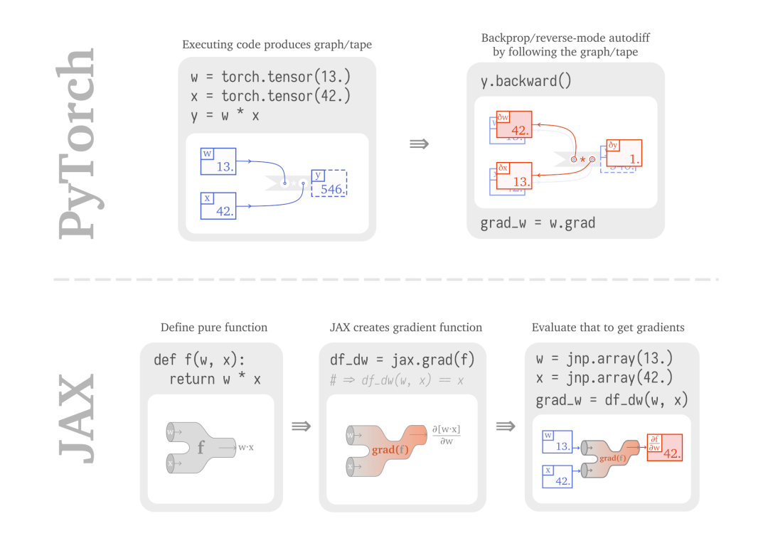
這樣一來，你進行編程和構建模型的方式就不一樣了。所以你可以使用 tape-based 的自動微分方法，并使用有狀態的對象。但是 Jax 可能讓你感到很吃驚，因為運行 grad() 函數的時候，它讓微分過程如同函數一樣。

也許你已經決定看看如 flax、trax 或 haiku 這些基于 Jax 的工具。在看 ResNet 等例子時，你會發現它和其他框架中的代碼不一樣。除了定義層、運行訓練外，底層的邏輯是什么樣的?這些小小的 numpy 程序是如何訓練了一個巨大的架構?

本文便是介紹 Jax 構建模型的教程，機器之心節選了其中的兩個部分：

• 快速回顧 PyTorch 上的 LSTM-LM 應用;
• 看看 PyTorch 風格的代碼(基于 mutate 狀態)，并了解純函數是如何構建模型的(Jax);

PyTorch 上的 LSTM 語言模型

我們首先用 PyTorch 實現 LSTM 語言模型，如下為代碼：

import torch 
class LSTMCell(torch.nn.Module):  
    def __init__(self, in_dim, out_dim):  
        super(LSTMCell, self).__init__()  
        self.weight_ih = torch.nn.Parameter(torch.rand(4*out_dim, in_dim))  
        self.weight_hh = torch.nn.Parameter(torch.rand(4*out_dim, out_dim))  
        self.bias = torch.nn.Parameter(torch.zeros(4*out_dim,))   
 
    def forward(self, inputs, h, c):  
        ifgo = self.weight_ih @ inputs + self.weight_hh @ h + self.bias  
        i, f, g, o = torch.chunk(ifgo, 4)  
        i = torch.sigmoid(i)  
        f = torch.sigmoid(f)  
        g = torch.tanh(g)  
        o = torch.sigmoid(o)  
        new_c = f * c + i * g  
        new_h = o * torch.tanh(new_c)  
        return (new_h, new_c) 

然后，我們基于這個 LSTM 神經元構建一個單層的網絡。這里會有一個嵌入層，它和可學習的 (h,c)0 會展示單個參數如何改變。

class LSTMLM(torch.nn.Module):  
    def __init__(self, vocab_size, dim=17):  
        super().__init__()  
        self.cell = LSTMCell(dim, dim)  
        self.embeddings = torch.nn.Parameter(torch.rand(vocab_size, dim))  
        self.c_0 = torch.nn.Parameter(torch.zeros(dim)) 
 
    @property  
    def hc_0(self):  
        return (torch.tanh(self.c_0), self.c_0) 
 
    def forward(self, seq, hc):  
         loss = torch.tensor(0.)  
          for idx in seq:  
              loss -= torch.log_softmax(self.embeddings @ hc[0], dim=-1)[idx]  
              hc = self.cell(self.embeddings[idx,:], *hc)  
          return loss, hc   
 
    def greedy_argmax(self, hc, length=6):  
        with torch.no_grad():  
            idxs = []  
            for i in range(length):  
                idx = torch.argmax(self.embeddings @ hc[0])  
                idxs.append(idx.item())  
                hc = self.cell(self.embeddings[idx,:], *hc)  
        return idxs 

構建后，進行訓練：

torch.manual_seed(0) 
# As training data, we will have indices of words/wordpieces/characters, 
# we just assume they are tokenized and integerized (toy example obviously). 
import jax.numpy as jnp 
vocab_size = 43 # prime trick! :) 
training_data = jnp.array([4, 8, 15, 16, 23, 42]) 
 
lm = LSTMLM(vocab_sizevocab_size=vocab_size) 
print("Sample before:", lm.greedy_argmax(lm.hc_0)) 
 
bptt_length = 3 # to illustrate hc.detach-ing 
 
for epoch in range(101):  
    hc = lm.hc_0  
    totalloss = 0.  
    for start in range(0, len(training_data), bptt_length):  
        batch = training_data[start:start+bptt_length]  
        loss, (h, c) = lm(batch, hc)  
        hc = (h.detach(), c.detach())  
        if epoch % 50 == 0:  
            totalloss += loss.item()  
        loss.backward()  
        for name, param in lm.named_parameters():  
            if param.grad is not None:  
                param.data -= 0.1 * param.grad  
                del param.grad  
     if totalloss:  
         print("Loss:", totalloss) 
          
print("Sample after:", lm.greedy_argmax(lm.hc_0)) 
Sample before: [42, 34, 34, 34, 34, 34] 
Loss: 25.953862190246582 
Loss: 3.7642268538475037 
Loss: 1.9537211656570435 
Sample after: [4, 8, 15, 16, 23, 42] 

可以看到，PyTorch 的代碼已經比較清楚了，但是還是有些問題。盡管我非常注意，但是還是要關注計算圖中的節點數量。那些中間節點需要在正確的時間被清除。

純函數

為了理解 JAX 如何處理這一問題，我們首先需要理解純函數的概念。如果你之前做過函數式編程，那你可能對以下概念比較熟悉：純函數就像數學中的函數或公式。它定義了如何從某些輸入值獲得輸出值。重要的是，它沒有「副作用」，即函數的任何部分都不會訪問或改變任何全局狀態。

我們在 Pytorch 中寫代碼時充滿了中間變量或狀態，而且這些狀態經常會改變，這使得推理和優化工作變得非常棘手。因此，JAX 選擇將程序員限制在純函數的范圍內，不讓上述情況發生。

在深入了解 JAX 之前，可以先看幾個純函數的例子。純函數必須滿足以下條件：

• 你在什么情況下執行函數、何時執行函數應該不影響輸出——只要輸入不變，輸出也應該不變;
• 無論我們將函數執行了 0 次、1 次還是多次，事后應該都是無法辨別的。

以下非純函數都至少違背了上述條件中的一條：

import random 
import time 
nr_executions = 0 
 
def pure_fn_1(x):  
    return 2 * x 
     
def pure_fn_2(xs):  
    ys = []  
    for x in xs:  
        # Mutating stateful variables *inside* the function is fine!  
        ys.append(2 * x)  
    return ys 
 
def impure_fn_1(xs):  
    # Mutating arguments has lasting consequences outside the function! :(  
    xs.append(sum(xs))  
    return xs 
 
def impure_fn_2(x):  
    # Very obviously mutating  
    global state is bad... global  
    nr_executions nr_executions += 1  
    return 2 * x 
 
def impure_fn_3(x):  
    # ...but just accessing it is, too, because now the function depends on the  
    # execution context!  
    return nr_executions * x 
 
def impure_fn_4(x):  
    # Things like IO are classic examples of impurity.  
    # All three of the following lines are violations of purity:  
    print("Hello!")  
    user_input = input()  
    execution_time = time.time()  
    return 2 * x 
 
def impure_fn_5(x):  
    # Which constraint does this violate? Both, actually! You access the current  
    # state of randomness *and* advance the number generator!  
    p = random.random()  
    return p * x 
Let's see a pure function that JAX operates on: the example from the intro figure. 
 
# (almost) 1-D linear regression 
def f(w, x):  
    return w * x 
 
print(f(13., 42.)) 
546.0 

目前為止還沒有出現什么狀況。JAX 現在允許你將下列函數轉換為另一個函數，不是返回結果，而是返回函數結果針對函數第一個參數的梯度。

import jax 
import jax.numpy as jnp 
 
# Gradient: with respect to weights! JAX uses the first argument by default. 
df_dw = jax.grad(f) 
 
def manual_df_dw(w, x):  
    return x 
     
assert df_dw(13., 42.) == manual_df_dw(13., 42.) 
 
print(df_dw(13., 42.)) 
42.0 

到目前為止，前面的所有內容你大概都在 JAX 的 README 文檔見過，內容也很合理。但怎么跳轉到類似 PyTorch 代碼里的那種大模塊呢?

首先，我們來添加一個偏置項，并嘗試將一維線性回歸變量包裝成一個我們習慣使用的對象——一種線性回歸「層」(LinearRegressor「layer」):

class LinearRegressor():  
    def __init__(self, w, b):  
    self.w = w  
    self.b = b  
     
    def predict(self, x):  
        return self.w * x + self.b  
         
    def rms(self, xs: jnp.ndarray, ys: jnp.ndarray):  
        return jnp.sqrt(jnp.sum(jnp.square(self.w * xs + self.b - ys))) 
         
my_regressor = LinearRegressor(13., 0.) 
 
# A kind of loss fuction, used for training 
xs = jnp.array([42.0]) 
ys = jnp.array([500.0]) 
print(my_regressor.rms(xs, ys)) 
 
# Prediction for test data 
print(my_regressor.predict(42.)) 
46.0 
546.0 

接下來要怎么利用梯度進行訓練呢?我們需要一個純函數，它將我們的模型權重作為函數的輸入參數，可能會像這樣：

def loss_fn(w, b, xs, ys):  
    my_regressor = LinearRegressor(w, b)  
    return my_regressor.rms(xsxs=xs, ysys=ys) 
     
# We use argnums=(0, 1) to tell JAX to give us 
# gradients wrt first and second parameter. 
grad_fn = jax.grad(loss_fn, argnums=(0, 1)) 
 
print(loss_fn(13., 0., xs, ys)) 
print(grad_fn(13., 0., xs, ys)) 
46.0 
(DeviceArray(42., dtype=float32), DeviceArray(1., dtype=float32)) 

你要說服自己這是對的。現在，這是可行的，但顯然，在 loss_fn 的定義部分枚舉所有參數是不可行的。

幸運的是，JAX 不僅可以對標量、向量、矩陣進行微分，還能對許多類似樹的數據結構進行微分。這種結構被稱為 pytree，包括 python dicts：

def loss_fn(params, xs, ys):  
    my_regressor = LinearRegressor(params['w'], params['b'])  
    return my_regressor.rms(xsxs=xs, ysys=ys) 
 
grad_fn = jax.grad(loss_fn) 
 
print(loss_fn({'w': 13., 'b': 0.}, xs, ys)) 
print(grad_fn({'w': 13., 'b': 0.}, xs, ys)) 
46.0 
{'b': DeviceArray(1., dtype=float32), 'w': DeviceArray(42., dtype=float32)}So this already looks nicer! We could write a training loop like this: 

現在看起來好多了!我們可以寫一個下面這樣的訓練循環：

params = {'w': 13., 'b': 0.} 
 
for _ in range(15):  
    print(loss_fn(params, xs, ys))  
    grads = grad_fn(params, xs, ys)  
    for name in params.keys():  
        params[name] -= 0.002 * grads[name] 
         
# Now, predict: 
LinearRegressor(params['w'], params['b']).predict(42.) 
46.0 
42.47003 
38.940002 
35.410034 
31.880066 
28.350098 
24.820068 
21.2901 
17.760132 
14.230164 
10.700165 
7.170166 
3.6401978 
0.110198975 
3.4197998 
DeviceArray(500.1102, dtype=float32) 

注意，現在已經可以使用更多的 JAX helper 來進行自我更新：由于參數和梯度擁有共同的(類似樹的)結構，我們可以想象將它們置于頂端，創造一個新樹，其值在任何地方都是這兩個樹的「組合」，如下所示：

def update_combiner(param, grad, lr=0.002):  
    return param - lr * grad 
     
params = jax.tree_multimap(update_combiner, params, grads) 
# instead of: 
# for name in params.keys(): 
# params[name] -= 0.1 * grads[name] 

參考鏈接：https://sjmielke.com/jax-purify.htm

【本文是51CTO專欄機構“機器之心”的原創譯文，微信公眾號“機器之心( id: almosthuman2014)”】 

戳這里，看該作者更多好文