[[328383]]

介紹：

• Boosting是一種集成技術，用于從多個弱分類器創建強分類器。 集成技術的一個眾所周知的例子是隨機森林(Random Forest)，它使用多個決策樹來創建一個隨機森林。

直覺：

• AdaBoost，Adaptive Boosting的縮寫，是第一個成功的針對二進制分類開發的Boosting算法。它是一種監督式機器學習算法，用于提高任何機器學習算法的性能。 最好與像決策樹這樣的弱學習者一起使用。 這些模型在分類問題上的準確性要高于隨機機會。

AdaBoost的概念很簡單：

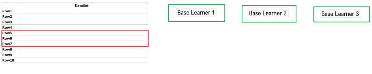
• 我們將把數據集傳遞給多個基礎學習者，每個基礎學習者將嘗試更正其前輩分類錯誤的記錄。

我們會將數據集(如下所示，所有行)傳遞給Base Learner1。所有被Base Learner 1誤分類的記錄(行5,6和7被錯誤分類)將被傳遞給Base Learner 2，類似地，所有Base分類器的錯誤分類記錄 學習者2將被傳遞給基本學習者3。最后，根據每個基本學習者的多數票，我們將對新記錄進行分類。

 

讓我們逐步了解AdaBoost分類器的實現：

步驟1：獲取數據集，并將初始權重分配給指定數據集中的所有樣本(行)。

W = 1 / n => 1/7，其中n是樣本數。

 

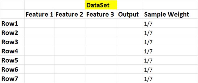
步驟2：我們將創建第一個基礎學習器。在AdaBoost中，我們將決策樹用作基礎學習器。這里要注意的是，我們將僅創建深度為1的決策樹，它們被稱為決策樹樁或樹樁。

 

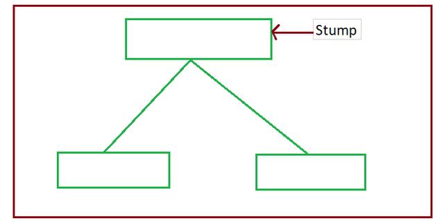
我們將為數據集的每個特征創建一個樹樁，就像在我們的例子中，我們將創建三個樹樁，每個特征一個。

步驟3：我們需要根據每個特征的熵值或吉尼系數，選擇任何基礎學習器模型(為特征1創建的基礎學習器1，為特征2創建的基礎學習器2，為特征3創建的基礎學習器3) (我在決策樹文章中已經討論了Ginni和熵)。

熵或吉尼系數值最小的基礎學習器，我們將為第一個基礎學習器模型選擇該模型。

第4步：我們需要找到在第3步中選擇的基本學習者模型正確分類了多少條記錄以及錯誤分類了多少條記錄。

我們必須找到所有錯誤分類的總錯誤，讓我們說我們是否正確分類了4條記錄而錯誤分類了1條記錄

Total Error =分類錯誤的記錄的樣本權重的總和。

因為我們只有1個錯誤，所以總錯誤= 1/7

步驟5：通過以下公式檢查樹樁的性能。

 

當我們將Total Error放入該公式時，我們將得到0.895的值(不要偷懶地將這些值進行計算)

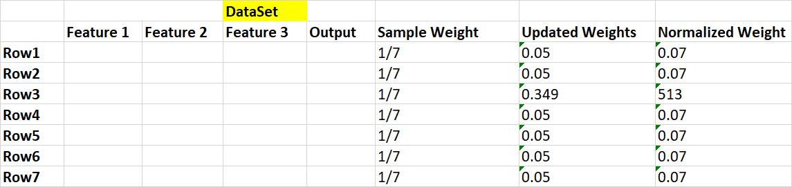
通過以下等式更新正確和錯誤分類的樣本(行)的樣本權重。

錯誤分類的樣本的新樣本權重=

 

 

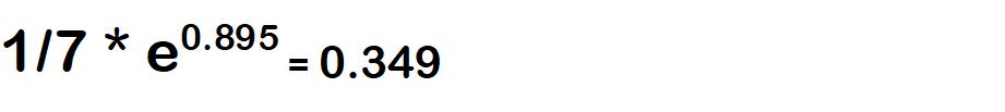
正確分類的樣本的新樣本權重=

 

 

 

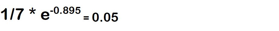
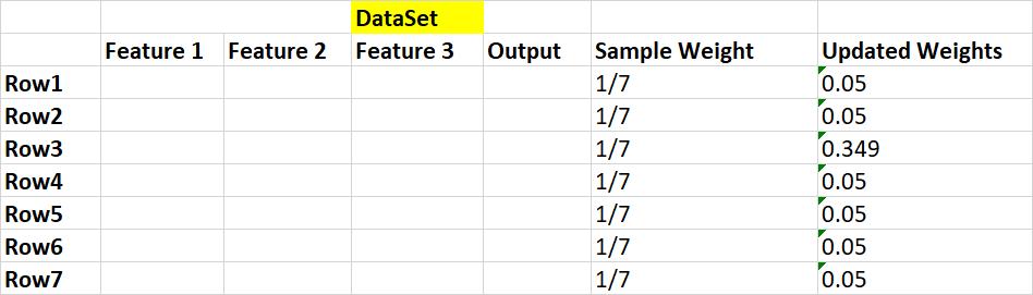
注意：我們假設第3行的分類不正確

步驟6：我們在這里考慮的要點是，當我們將所有樣本權重相加時，它等于1，但如果更新了權重，則總和不等于1。因此，我們將每個更新的權重除以總和，然后歸一化 值為1。

更新權重的總和是0.68

 

第7步：我們將通過刪除"樣品重量"和"更新重量"功能來創建數據集，并將每個樣品(行)分配到一個桶中。

 

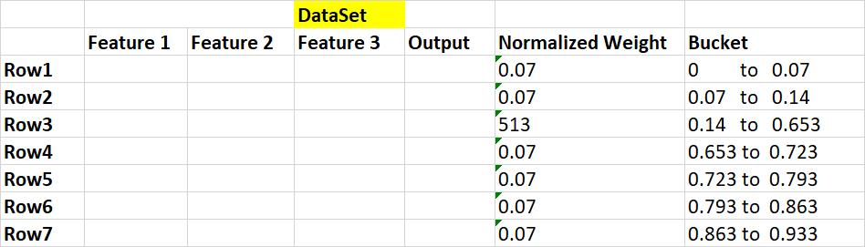
步驟8：建立新的資料集。 為此，我們必須從0到1(對于每個樣本(行))中隨機選擇一個值，然后選擇該樣本，該樣本在" Bucket"下掉落，并將該樣本保留在" NEW DATASET"中。 由于分類錯誤的記錄具有較大的存儲桶大小，因此選擇該記錄的可能性非常高。

 

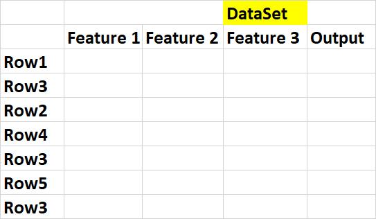
我們在這里可以看到，由于數據桶大小比其他行大，因此已在我們的數據集中選擇了3次錯誤分類的record(Row3)。

第9步：為下一個樹樁(基礎學習者2，基礎學習者3)獲取此新數據集，并按照步驟1至8進行所有功能。

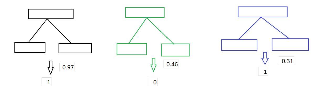
Adaboost模型通過讓森林中的每棵樹對樣本進行分類來進行預測。然后，根據樹木的決策將它們分成幾組。現在，對于每組，我們對各樹中每棵樹的重要性進行累加。 整個森林的數量由總和最大的群體決定。下圖。

 

Adaboost分類器的逐步Python代碼：

In [1]: 
#General idea behind boosting methods is to train predictors sequentially,each trying to correct its predecessor 
 
# AdaBoost Classifier Example In Python 
# Step 1: Initialize the sample weights 
# Step 2: Build a decision tree with each feature, classify the data and evaluate the result 
# Step 3: Calculate the significance of the tree in the final classification 
# Step 4: Update the sample weights so that the next decision tree will take the errors made by the preceding decision tree into account 
# Step 5: Form a new dataset 
# Step 6: Repeat steps 2 through 5 until the number of iterations equals the number specified by the hyperparameter (i.e. number of estimators) 
# Step 7: Use the forest of decision trees to make predictions on data outside of the training set 
In [2]: 
from sklearn.ensemble import AdaBoostClassifier 
from sklearn.tree import DecisionTreeClassifier 
from sklearn.datasets import load_breast_cancer 
import pandas as pd 
import numpy as np 
import seaborn as sns 
import matplotlib.pyplot as plt 
from sklearn.model_selection import train_test_split 
from sklearn.metrics import confusion_matrix,accuracy_score 
from sklearn.preprocessing import LabelEncoder 
import warnings 
warnings.filterwarnings('ignore') 
In [3]: 
cancer_data=load_breast_cancer() 
In [4]: 
X=pd.DataFrame(cancer_data.data,columns=cancer_data.feature_names) 
In [5]: 
y = pd.Categorical.from_codes(cancer_data.target, cancer_data.target_names) 
In [6]: 
#y=pd.DataFrame(y,columns=['Cancer_Target']) 
Data Preprocessing 
In [7]: 
X.describe() 
Out[7]: 
mean radius mean texture    mean perimeter  mean area   mean smoothness mean compactness    mean concavity  mean concave points mean symmetry   mean fractal dimension  ... worst radius    worst texture   worst perimeter worst area  worst smoothness    worst compactness   worst concavity worst concave points    worst symmetry  worst fractal dimension 
count   569.000000  569.000000  569.000000  569.000000  569.000000  569.000000  569.000000  569.000000  569.000000  569.000000  ... 569.000000  569.000000  569.000000  569.000000  569.000000  569.000000  569.000000  569.000000  569.000000  569.000000 
mean    14.127292   19.289649   91.969033   654.889104  0.096360    0.104341    0.088799    0.048919    0.181162    0.062798    ... 16.269190   25.677223   107.261213  880.583128  0.132369    0.254265    0.272188    0.114606    0.290076    0.083946 
std 3.524049    4.301036    24.298981   351.914129  0.014064    0.052813    0.079720    0.038803    0.027414    0.007060    ... 4.833242    6.146258    33.602542   569.356993  0.022832    0.157336    0.208624    0.065732    0.061867    0.018061 
min 6.981000    9.710000    43.790000   143.500000  0.052630    0.019380    0.000000    0.000000    0.106000    0.049960    ... 7.930000    12.020000   50.410000   185.200000  0.071170    0.027290    0.000000    0.000000    0.156500    0.055040 
25% 11.700000   16.170000   75.170000   420.300000  0.086370    0.064920    0.029560    0.020310    0.161900    0.057700    ... 13.010000   21.080000   84.110000   515.300000  0.116600    0.147200    0.114500    0.064930    0.250400    0.071460 
50% 13.370000   18.840000   86.240000   551.100000  0.095870    0.092630    0.061540    0.033500    0.179200    0.061540    ... 14.970000   25.410000   97.660000   686.500000  0.131300    0.211900    0.226700    0.099930    0.282200    0.080040 
75% 15.780000   21.800000   104.100000  782.700000  0.105300    0.130400    0.130700    0.074000    0.195700    0.066120    ... 18.790000   29.720000   125.400000  1084.000000 0.146000    0.339100    0.382900    0.161400    0.317900    0.092080 
max 28.110000   39.280000   188.500000  2501.000000 0.163400    0.345400    0.426800    0.201200    0.304000    0.097440    ... 36.040000   49.540000   251.200000  4254.000000 0.222600    1.058000    1.252000    0.291000    0.663800    0.207500 
8 rows × 30 columns 
 
In [8]: 
X.isnull().count() 
Out[8]: 
mean radius                569 
mean texture               569 
mean perimeter             569 
mean area                  569 
mean smoothness            569 
mean compactness           569 
mean concavity             569 
mean concave points        569 
mean symmetry              569 
mean fractal dimension     569 
radius error               569 
texture error              569 
perimeter error            569 
area error                 569 
smoothness error           569 
compactness error          569 
concavity error            569 
concave points error       569 
symmetry error             569 
fractal dimension error    569 
worst radius               569 
worst texture              569 
worst perimeter            569 
worst area                 569 
worst smoothness           569 
worst compactness          569 
worst concavity            569 
worst concave points       569 
worst symmetry             569 
worst fractal dimension    569 
dtype: int64 
In [9]: 
def heatMap(df): 
    #Create Correlation df 
    corr = X.corr() 
    #Plot figsize 
    fig, ax = plt.subplots(figsize=(25, 25)) 
    #Generate Color Map 
    colormap = sns.diverging_palette(220, 10, as_cmap=True) 
    #Generate Heat Map, allow annotations and place floats in map 
    sns.heatmap(corr, cmap=colormap, annot=True, fmt=".2f") 
    #Apply xticks 
    plt.xticks(range(len(corr.columns)), corr.columns); 
    #Apply yticks 
    plt.yticks(range(len(corr.columns)), corr.columns) 
    #show plot 
    plt.show() 
In [10]: 
heatMap(X) 
 
All the above correlated features can be dropped 
In [11]: 
X.boxplot(figsize=(10,15)) 
Out[11]: 
<matplotlib.axes._subplots.AxesSubplot at 0x1e1a0eb7fd0> 
 
In [12]: 
le=LabelEncoder() 
In [13]: 
y=pd.Series(le.fit_transform(y)) 
Data Split and Model Initialization 
In [14]: 
X_train,X_test,y_train,y_test=train_test_split(X,y,test_size=0.20,random_state=42) 
In [15]: 
adaboost=AdaBoostClassifier(DecisionTreeClassifier(max_depth=1),n_estimators=200) 
In [16]: 
adaboost.fit(X_train,y_train) 
Out[16]: 
AdaBoostClassifier(algorithm='SAMME.R', 
          base_estimator=DecisionTreeClassifier(class_weight=None, criterion='gini', max_depth=1, 
            max_features=None, max_leaf_nodes=None, 
            min_impurity_decrease=0.0, min_impurity_split=None, 
            min_samples_leaf=1, min_samples_split=2, 
            min_weight_fraction_leaf=0.0, presort=False, random_state=None, 
            splitter='best'), 
          learning_rate=1.0, n_estimators=200, random_state=None) 
In [17]: 
adaboost.score(X_train,y_train) 
Out[17]: 
1.0 
In [18]: 
adaboost.score(X_test,y_test) 
Out[18]: 
0.9736842105263158 
In [19]: 
y_pred=adaboost.predict(X_test) 
In [20]: 
y_pred 
Out[20]: 
array([0, 1, 1, 0, 0, 1, 1, 1, 1, 0, 0, 1, 0, 1, 0, 1, 0, 0, 0, 1, 0, 0, 
       1, 0, 0, 0, 0, 0, 0, 1, 0, 0, 0, 0, 0, 0, 1, 0, 1, 0, 0, 1, 0, 0, 
       0, 0, 0, 0, 0, 0, 1, 1, 0, 0, 0, 0, 0, 1, 1, 0, 0, 1, 1, 0, 0, 0, 
       1, 1, 0, 0, 1, 1, 0, 1, 0, 0, 0, 0, 0, 0, 1, 0, 1, 1, 1, 1, 1, 1, 
       0, 0, 0, 0, 0, 0, 0, 0, 1, 1, 0, 1, 1, 0, 1, 1, 0, 0, 0, 1, 0, 0, 
       1, 0, 0, 1]) 
Result Visualization 
In [21]: 
cm=confusion_matrix(y_test,y_pred) 
print('Confusion Matrix\n {} '.format(cm)) 
Confusion Matrix 
 [[70  1] 
 [ 2 41]]  
In [22]: 
ax= plt.subplot() 
sns.heatmap(cm, annot=True, ax = ax); 
# labels, title and ticks 
ax.set_xlabel('Predicted labels'); 
ax.set_ylabel('True labels');  
ax.set_title('Confusion Matrix'); 
 
In [23]: 
acc=accuracy_score(y_test,y_pred) 
print('Model Accuracy is {} % '.format(round(acc,3))) 
Model Accuracy is 0.974 %  

AdaBoost分類器的優點：

• AdaBoost可用于提高弱分類器的準確性，從而使其更靈活。 現在，它已擴展到二進制分類之外，并且還發現了文本和圖像分類中的用例。
• AdaBoost具有很高的精度。
• 不同的分類算法可以用作弱分類器。

缺點：

• 提升技巧是逐步學習的，確保您擁有高質量的數據非常重要。
• AdaBoost對噪聲數據和異常值也非常敏感，因此，如果您打算使用AdaBoost，則強烈建議消除它們。
• AdaBoost還被證明比XGBoost慢。

結論：在本文中，我們討論了理解AdaBoost算法的各種方法.AdaBoost就像是一個恩賜，如果正確使用它可以提高分類算法的準確性。

希望您喜歡我的文章。請鼓掌(最多50次)，這會激發我寫更多的文章。