從零開始使用 Nadam 進(jìn)行梯度下降優(yōu)化
梯度下降是一種優(yōu)化算法,遵循目標(biāo)函數(shù)的負(fù)梯度以定位函數(shù)的最小值。
梯度下降的局限性在于,如果梯度變?yōu)槠教够虼笄剩阉鞯倪M(jìn)度可能會(huì)減慢。可以將動(dòng)量添加到梯度下降中,該下降合并了一些慣性以進(jìn)行更新。可以通過合并預(yù)計(jì)的新位置而非當(dāng)前位置的梯度(稱為Nesterov的加速梯度(NAG)或Nesterov動(dòng)量)來進(jìn)一步改善此效果。
梯度下降的另一個(gè)限制是,所有輸入變量都使用單個(gè)步長(zhǎng)(學(xué)習(xí)率)。對(duì)梯度下降的擴(kuò)展,如自適應(yīng)運(yùn)動(dòng)估計(jì)(Adam)算法,該算法對(duì)每個(gè)輸入變量使用單獨(dú)的步長(zhǎng),但可能會(huì)導(dǎo)致步長(zhǎng)迅速減小到非常小的值。Nesterov加速的自適應(yīng)矩估計(jì)或Nadam是Adam算法的擴(kuò)展,該算法結(jié)合了Nesterov動(dòng)量,可以使優(yōu)化算法具有更好的性能。
在本教程中,您將發(fā)現(xiàn)如何從頭開始使用Nadam進(jìn)行梯度下降優(yōu)化。完成本教程后,您將知道:
- 梯度下降是一種優(yōu)化算法,它使用目標(biāo)函數(shù)的梯度來導(dǎo)航搜索空間。
- 納丹(Nadam)是亞當(dāng)(Adam)版本的梯度下降的擴(kuò)展,其中包括了內(nèi)斯特羅夫的動(dòng)量。
- 如何從頭開始實(shí)現(xiàn)Nadam優(yōu)化算法并將其應(yīng)用于目標(biāo)函數(shù)并評(píng)估結(jié)果。
教程概述
本教程分為三個(gè)部分:他們是:
- 梯度下降
- Nadam優(yōu)化算法
- 娜達(dá)姆(Nadam)的梯度下降
- 二維測(cè)試問題
- Nadam的梯度下降優(yōu)化
- 可視化的Nadam優(yōu)化
梯度下降
梯度下降是一種優(yōu)化算法。它在技術(shù)上稱為一階優(yōu)化算法,因?yàn)樗鞔_利用了目標(biāo)目標(biāo)函數(shù)的一階導(dǎo)數(shù)。
一階導(dǎo)數(shù),或簡(jiǎn)稱為“導(dǎo)數(shù)”,是目標(biāo)函數(shù)在特定點(diǎn)(例如,點(diǎn))上的變化率或斜率。用于特定輸入。
如果目標(biāo)函數(shù)采用多個(gè)輸入變量,則將其稱為多元函數(shù),并且可以將輸入變量視為向量。反過來,多元目標(biāo)函數(shù)的導(dǎo)數(shù)也可以視為向量,通常稱為梯度。
梯度:多元目標(biāo)函數(shù)的一階導(dǎo)數(shù)。
對(duì)于特定輸入,導(dǎo)數(shù)或梯度指向目標(biāo)函數(shù)最陡峭的上升方向。梯度下降是指一種最小化優(yōu)化算法,該算法遵循目標(biāo)函數(shù)的下坡梯度負(fù)值來定位函數(shù)的最小值。
梯度下降算法需要一個(gè)正在優(yōu)化的目標(biāo)函數(shù)和該目標(biāo)函數(shù)的導(dǎo)數(shù)函數(shù)。目標(biāo)函數(shù)f()返回給定輸入集合的分?jǐn)?shù),導(dǎo)數(shù)函數(shù)f'()給出給定輸入集合的目標(biāo)函數(shù)的導(dǎo)數(shù)。梯度下降算法需要問題中的起點(diǎn)(x),例如輸入空間中的隨機(jī)選擇點(diǎn)。
假設(shè)我們正在最小化目標(biāo)函數(shù),然后計(jì)算導(dǎo)數(shù)并在輸入空間中采取一步,這將導(dǎo)致目標(biāo)函數(shù)下坡運(yùn)動(dòng)。首先通過計(jì)算輸入空間中要移動(dòng)多遠(yuǎn)的距離來進(jìn)行下坡運(yùn)動(dòng),計(jì)算方法是將步長(zhǎng)(稱為alpha或?qū)W習(xí)率)乘以梯度。然后從當(dāng)前點(diǎn)減去該值,以確保我們逆梯度移動(dòng)或向下移動(dòng)目標(biāo)函數(shù)。
- x(t)= x(t-1)–step* f'(x(t))
在給定點(diǎn)的目標(biāo)函數(shù)越陡峭,梯度的大小越大,反過來,在搜索空間中采取的步伐也越大。使用步長(zhǎng)超參數(shù)來縮放步長(zhǎng)的大小。
步長(zhǎng):超參數(shù),用于控制算法每次迭代相對(duì)于梯度在搜索空間中移動(dòng)多遠(yuǎn)。
如果步長(zhǎng)太小,則搜索空間中的移動(dòng)將很小,并且搜索將花費(fèi)很長(zhǎng)時(shí)間。如果步長(zhǎng)太大,則搜索可能會(huì)在搜索空間附近反彈并跳過最優(yōu)值。
現(xiàn)在我們已經(jīng)熟悉了梯度下降優(yōu)化算法,接下來讓我們看一下Nadam算法。
Nadam優(yōu)化算法
Nesterov加速的自適應(yīng)動(dòng)量估計(jì)或Nadam算法是對(duì)自適應(yīng)運(yùn)動(dòng)估計(jì)(Adam)優(yōu)化算法的擴(kuò)展,添加了Nesterov的加速梯度(NAG)或Nesterov動(dòng)量,這是一種改進(jìn)的動(dòng)量。更廣泛地講,Nadam算法是對(duì)梯度下降優(yōu)化算法的擴(kuò)展。Timothy Dozat在2016年的論文“將Nesterov動(dòng)量整合到Adam中”中描述了該算法。盡管論文的一個(gè)版本是在2015年以同名斯坦福項(xiàng)目報(bào)告的形式編寫的。動(dòng)量將梯度的指數(shù)衰減移動(dòng)平均值(第一矩)添加到梯度下降算法中。這具有消除嘈雜的目標(biāo)函數(shù)和提高收斂性的影響。Adam是梯度下降的擴(kuò)展,它增加了梯度的第一和第二矩,并針對(duì)正在優(yōu)化的每個(gè)參數(shù)自動(dòng)調(diào)整學(xué)習(xí)率。NAG是動(dòng)量的擴(kuò)展,其中動(dòng)量的更新是使用對(duì)參數(shù)的預(yù)計(jì)更新量而不是實(shí)際當(dāng)前變量值的梯度來執(zhí)行的。在某些情況下,這樣做的效果是在找到最佳位置時(shí)減慢了搜索速度,而不是過沖。
納丹(Nadam)是對(duì)亞當(dāng)(Adam)的擴(kuò)展,它使用NAG動(dòng)量代替經(jīng)典動(dòng)量。讓我們逐步介紹該算法的每個(gè)元素。Nadam使用衰減步長(zhǎng)(alpha)和一階矩(mu)超參數(shù)來改善性能。為了簡(jiǎn)單起見,我們暫時(shí)將忽略此方面,并采用恒定值。首先,對(duì)于搜索中要優(yōu)化的每個(gè)參數(shù),我們必須保持梯度的第一矩和第二矩,分別稱為m和n。在搜索開始時(shí)將它們初始化為0.0。
- m = 0
- n = 0
該算法在從t = 1開始的時(shí)間t內(nèi)迭代執(zhí)行,并且每次迭代都涉及計(jì)算一組新的參數(shù)值x,例如。從x(t-1)到x(t)。如果我們專注于更新一個(gè)參數(shù),這可能很容易理解該算法,該算法概括為通過矢量運(yùn)算來更新所有參數(shù)。首先,計(jì)算當(dāng)前時(shí)間步長(zhǎng)的梯度(偏導(dǎo)數(shù))。
- g(t)= f'(x(t-1))
接下來,使用梯度和超參數(shù)“ mu”更新第一時(shí)刻。
- m(t)=mu* m(t-1)+(1 –mu)* g(t)
然后使用“ nu”超參數(shù)更新第二時(shí)刻。
- n(t)= nu * n(t-1)+(1 – nu)* g(t)^ 2
接下來,使用Nesterov動(dòng)量對(duì)第一時(shí)刻進(jìn)行偏差校正。
- mhat =(mu * m(t)/(1 – mu))+((1 – mu)* g(t)/(1 – mu))
然后對(duì)第二個(gè)時(shí)刻進(jìn)行偏差校正。注意:偏差校正是Adam的一個(gè)方面,它與在搜索開始時(shí)將第一時(shí)刻和第二時(shí)刻初始化為零這一事實(shí)相反。
- nhat = nu * n(t)/(1 – nu)
最后,我們可以為該迭代計(jì)算參數(shù)的值。
- x(t)= x(t-1)– alpha /(sqrt(nhat)+ eps)* mhat
其中alpha是步長(zhǎng)(學(xué)習(xí)率)超參數(shù),sqrt()是平方根函數(shù),eps(epsilon)是一個(gè)較小的值,如1e-8,以避免除以零誤差。
回顧一下,該算法有三個(gè)超參數(shù)。他們是:
- alpha:初始步長(zhǎng)(學(xué)習(xí)率),典型值為0.002。
- mu:第一時(shí)刻的衰減因子(Adam中的beta1),典型值為0.975。
- nu:第二時(shí)刻的衰減因子(Adam中的beta2),典型值為0.999。
就是這樣。接下來,讓我們看看如何在Python中從頭開始實(shí)現(xiàn)該算法。
娜達(dá)姆(Nadam)的梯度下降
在本節(jié)中,我們將探索如何使用Nadam動(dòng)量實(shí)現(xiàn)梯度下降優(yōu)化算法。
二維測(cè)試問題
首先,讓我們定義一個(gè)優(yōu)化函數(shù)。我們將使用一個(gè)簡(jiǎn)單的二維函數(shù),該函數(shù)將每個(gè)維的輸入平方,并定義有效輸入的范圍(從-1.0到1.0)。下面的Objective()函數(shù)實(shí)現(xiàn)了此功能
- # objective function
- def objective(x, y):
- return x**2.0 + y**2.0
我們可以創(chuàng)建數(shù)據(jù)集的三維圖,以了解響應(yīng)面的曲率。下面列出了繪制目標(biāo)函數(shù)的完整示例。
- # 3d plot of the test function
- from numpy import arange
- from numpy import meshgrid
- from matplotlib import pyplot
- # objective function
- def objective(x, y):
- return x**2.0 + y**2.0
- # define range for input
- r_min, r_max = -1.0, 1.0
- # sample input range uniformly at 0.1 increments
- xaxis = arange(r_min, r_max, 0.1)
- yaxis = arange(r_min, r_max, 0.1)
- # create a mesh from the axis
- x, y = meshgrid(xaxis, yaxis)
- # compute targets
- results = objective(x, y)
- # create a surface plot with the jet color scheme
- figure = pyplot.figure()
- axis = figure.gca(projection='3d')
- axis.plot_surface(x, y, results, cmap='jet')
- # show the plot
- pyplot.show()
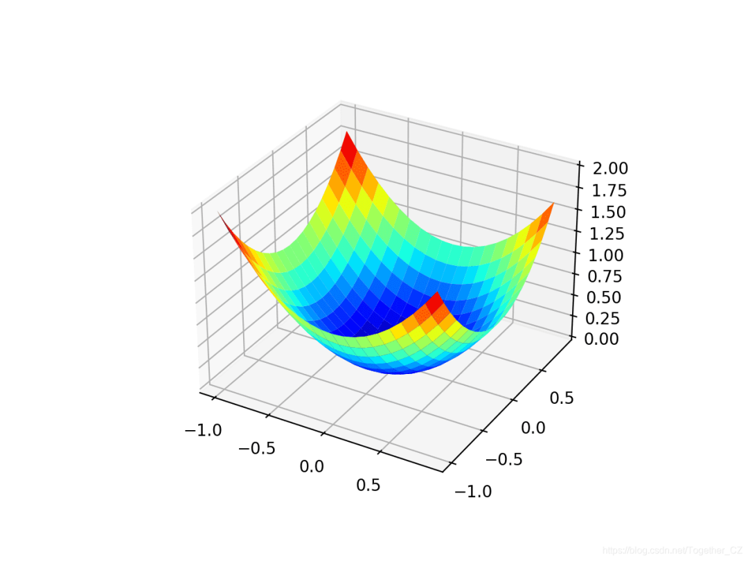
運(yùn)行示例將創(chuàng)建目標(biāo)函數(shù)的三維表面圖。我們可以看到全局最小值為f(0,0)= 0的熟悉的碗形狀。
我們還可以創(chuàng)建函數(shù)的二維圖。這在以后要繪制搜索進(jìn)度時(shí)會(huì)很有幫助。下面的示例創(chuàng)建目標(biāo)函數(shù)的輪廓圖。
- # contour plot of the test function
- from numpy import asarray
- from numpy import arange
- from numpy import meshgrid
- from matplotlib import pyplot
- # objective function
- def objective(x, y):
- return x**2.0 + y**2.0
- # define range for input
- bounds = asarray([[-1.0, 1.0], [-1.0, 1.0]])
- # sample input range uniformly at 0.1 increments
- xaxis = arange(bounds[0,0], bounds[0,1], 0.1)
- yaxis = arange(bounds[1,0], bounds[1,1], 0.1)
- # create a mesh from the axis
- x, y = meshgrid(xaxis, yaxis)
- # compute targets
- results = objective(x, y)
- # create a filled contour plot with 50 levels and jet color scheme
- pyplot.contourf(x, y, results, levels=50, cmap='jet')
- # show the plot
- pyplot.show()
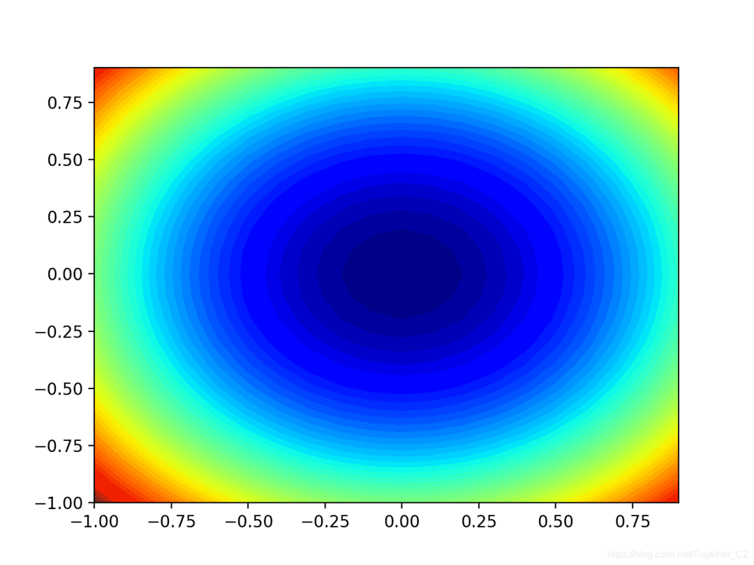
運(yùn)行示例將創(chuàng)建目標(biāo)函數(shù)的二維輪廓圖。我們可以看到碗的形狀被壓縮為以顏色漸變顯示的輪廓。我們將使用該圖來繪制在搜索過程中探索的特定點(diǎn)。
現(xiàn)在我們有了一個(gè)測(cè)試目標(biāo)函數(shù),讓我們看一下如何實(shí)現(xiàn)Nadam優(yōu)化算法。
Nadam的梯度下降優(yōu)化
我們可以將Nadam的梯度下降應(yīng)用于測(cè)試問題。首先,我們需要一個(gè)函數(shù)來計(jì)算此函數(shù)的導(dǎo)數(shù)。
x ^ 2的導(dǎo)數(shù)在每個(gè)維度上均為x * 2。
- f(x)= x ^ 2
- f'(x)= x * 2
derived()函數(shù)在下面實(shí)現(xiàn)了這一點(diǎn)。
- # derivative of objective function
- def derivative(x, y):
- return asarray([x * 2.0, y * 2.0])
接下來,我們可以使用Nadam實(shí)現(xiàn)梯度下降優(yōu)化。首先,我們可以選擇問題范圍內(nèi)的隨機(jī)點(diǎn)作為搜索的起點(diǎn)。假定我們有一個(gè)數(shù)組,該數(shù)組定義搜索范圍,每個(gè)維度一行,并且第一列定義最小值,第二列定義維度的最大值。
- # generate an initial point
- x = bounds[:, 0] + rand(len(bounds)) * (bounds[:, 1] - bounds[:, 0])
- score = objective(x[0], x[1])
接下來,我們需要初始化力矩矢量。
- # initialize decaying moving averages
- m = [0.0 for _ in range(bounds.shape[0])]
- n = [0.0 for _ in range(bounds.shape[0])]
然后,我們運(yùn)行由“ n_iter”超參數(shù)定義的算法的固定迭代次數(shù)。
- ...
- # run iterations of gradient descent
- for t in range(n_iter):
- ...
第一步是計(jì)算當(dāng)前參數(shù)集的導(dǎo)數(shù)。
- ...
- # calculate gradient g(t)
- g = derivative(x[0], x[1])
接下來,我們需要執(zhí)行Nadam更新計(jì)算。為了提高可讀性,我們將使用命令式編程樣式來一次執(zhí)行一個(gè)變量的這些計(jì)算。在實(shí)踐中,我建議使用NumPy向量運(yùn)算以提高效率。
- ...
- # build a solution one variable at a time
- for i in range(x.shape[0]):
- ...
首先,我們需要計(jì)算力矩矢量。
- # m(t) = mu * m(t-1) + (1 - mu) * g(t)
- m[i] = mu * m[i] + (1.0 - mu) * g[i]
然后是第二個(gè)矩向量。
- # nhat = nu * n(t) / (1 - nu)
- nhat = nu * n[i] / (1.0 - nu)
- # n(t) = nu * n(t-1) + (1 - nu) * g(t)^2
- n[i] = nu * n[i] + (1.0 - nu) * g[i]**2
然后是經(jīng)過偏差校正的內(nèi)斯特羅夫動(dòng)量。
- # mhat = (mu * m(t) / (1 - mu)) + ((1 - mu) * g(t) / (1 - mu))
- mhat = (mu * m[i] / (1.0 - mu)) + ((1 - mu) * g[i] / (1.0 - mu))
偏差校正的第二時(shí)刻。
- # nhat = nu * n(t) / (1 - nu)
- nhat = nu * n[i] / (1.0 - nu)
最后更新參數(shù)。
- # x(t) = x(t-1) - alpha / (sqrt(nhat) + eps) * mhat
- x[i] = x[i] - alpha / (sqrt(nhat) + eps) * mhat
然后,針對(duì)要優(yōu)化的每個(gè)參數(shù)重復(fù)此操作。在迭代結(jié)束時(shí),我們可以評(píng)估新的參數(shù)值并報(bào)告搜索的性能。
- # evaluate candidate point
- score = objective(x[0], x[1])
- # report progress
- print('>%d f(%s) = %.5f' % (t, x, score))
我們可以將所有這些結(jié)合到一個(gè)名為nadam()的函數(shù)中,該函數(shù)采用目標(biāo)函數(shù)和派生函數(shù)的名稱以及算法超參數(shù),并返回在搜索及其評(píng)估結(jié)束時(shí)找到的最佳解決方案。
- # gradient descent algorithm with nadam
- def nadam(objective, derivative, bounds, n_iter, alpha, mu, nu, eps=1e-8):
- # generate an initial point
- x = bounds[:, 0] + rand(len(bounds)) * (bounds[:, 1] - bounds[:, 0])
- score = objective(x[0], x[1])
- # initialize decaying moving averages
- m = [0.0 for _ in range(bounds.shape[0])]
- n = [0.0 for _ in range(bounds.shape[0])]
- # run the gradient descent
- for t in range(n_iter):
- # calculate gradient g(t)
- g = derivative(x[0], x[1])
- # build a solution one variable at a time
- for i in range(bounds.shape[0]):
- # m(t) = mu * m(t-1) + (1 - mu) * g(t)
- m[i] = mu * m[i] + (1.0 - mu) * g[i]
- # n(t) = nu * n(t-1) + (1 - nu) * g(t)^2
- n[i] = nu * n[i] + (1.0 - nu) * g[i]**2
- # mhat = (mu * m(t) / (1 - mu)) + ((1 - mu) * g(t) / (1 - mu))
- mhat = (mu * m[i] / (1.0 - mu)) + ((1 - mu) * g[i] / (1.0 - mu))
- # nhat = nu * n(t) / (1 - nu)
- nhat = nu * n[i] / (1.0 - nu)
- # x(t) = x(t-1) - alpha / (sqrt(nhat) + eps) * mhat
- x[i] = x[i] - alpha / (sqrt(nhat) + eps) * mhat
- # evaluate candidate point
- score = objective(x[0], x[1])
- # report progress
- print('>%d f(%s) = %.5f' % (t, x, score))
- return [x, score]
然后,我們可以定義函數(shù)和超參數(shù)的界限,并調(diào)用函數(shù)執(zhí)行優(yōu)化。在這種情況下,我們將運(yùn)行該算法進(jìn)行50次迭代,初始alpha為0.02,μ為0.8,nu為0.999,這是經(jīng)過一點(diǎn)點(diǎn)反復(fù)試驗(yàn)后發(fā)現(xiàn)的。
- # seed the pseudo random number generator
- seed(1)
- # define range for input
- bounds = asarray([[-1.0, 1.0], [-1.0, 1.0]])
- # define the total iterations
- n_iter = 50
- # steps size
- alpha = 0.02
- # factor for average gradient
- mu = 0.8
- # factor for average squared gradient
- nu = 0.999
- # perform the gradient descent search with nadam
- best, score = nadam(objective, derivative, bounds, n_iter, alpha, mu, nu)
運(yùn)行結(jié)束時(shí),我們將報(bào)告找到的最佳解決方案。
- # summarize the result
- print('Done!')
- print('f(%s) = %f' % (best, score))
綜合所有這些,下面列出了適用于我們的測(cè)試問題的Nadam梯度下降的完整示例。
- # gradient descent optimization with nadam for a two-dimensional test function
- from math import sqrt
- from numpy import asarray
- from numpy.random import rand
- from numpy.random import seed
- # objective function
- def objective(x, y):
- return x**2.0 + y**2.0
- # derivative of objective function
- def derivative(x, y):
- return asarray([x * 2.0, y * 2.0])
- # gradient descent algorithm with nadam
- def nadam(objective, derivative, bounds, n_iter, alpha, mu, nu, eps=1e-8):
- # generate an initial point
- x = bounds[:, 0] + rand(len(bounds)) * (bounds[:, 1] - bounds[:, 0])
- score = objective(x[0], x[1])
- # initialize decaying moving averages
- m = [0.0 for _ in range(bounds.shape[0])]
- n = [0.0 for _ in range(bounds.shape[0])]
- # run the gradient descent
- for t in range(n_iter):
- # calculate gradient g(t)
- g = derivative(x[0], x[1])
- # build a solution one variable at a time
- for i in range(bounds.shape[0]):
- # m(t) = mu * m(t-1) + (1 - mu) * g(t)
- m[i] = mu * m[i] + (1.0 - mu) * g[i]
- # n(t) = nu * n(t-1) + (1 - nu) * g(t)^2
- n[i] = nu * n[i] + (1.0 - nu) * g[i]**2
- # mhat = (mu * m(t) / (1 - mu)) + ((1 - mu) * g(t) / (1 - mu))
- mhat = (mu * m[i] / (1.0 - mu)) + ((1 - mu) * g[i] / (1.0 - mu))
- # nhat = nu * n(t) / (1 - nu)
- nhat = nu * n[i] / (1.0 - nu)
- # x(t) = x(t-1) - alpha / (sqrt(nhat) + eps) * mhat
- x[i] = x[i] - alpha / (sqrt(nhat) + eps) * mhat
- # evaluate candidate point
- score = objective(x[0], x[1])
- # report progress
- print('>%d f(%s) = %.5f' % (t, x, score))
- return [x, score]
- # seed the pseudo random number generator
- seed(1)
- # define range for input
- bounds = asarray([[-1.0, 1.0], [-1.0, 1.0]])
- # define the total iterations
- n_iter = 50
- # steps size
- alpha = 0.02
- # factor for average gradient
- mu = 0.8
- # factor for average squared gradient
- nu = 0.999
- # perform the gradient descent search with nadam
- best, score = nadam(objective, derivative, bounds, n_iter, alpha, mu, nu)
- print('Done!')
- print('f(%s) = %f' % (best, score))
運(yùn)行示例將優(yōu)化算法和Nadam應(yīng)用于我們的測(cè)試問題,并報(bào)告算法每次迭代的搜索性能。
注意:由于算法或評(píng)估程序的隨機(jī)性,或者數(shù)值精度的差異,您的結(jié)果可能會(huì)有所不同。考慮運(yùn)行該示例幾次并比較平均結(jié)果。
在這種情況下,我們可以看到在大約44次搜索迭代后找到了接近最佳的解決方案,輸入值接近0.0和0.0,評(píng)估為0.0。
- >40 f([ 5.07445337e-05 -3.32910019e-03]) = 0.00001
- >41 f([-1.84325171e-05 -3.00939427e-03]) = 0.00001
- >42 f([-6.78814472e-05 -2.69839367e-03]) = 0.00001
- >43 f([-9.88339249e-05 -2.40042096e-03]) = 0.00001
- >44 f([-0.00011368 -0.00211861]) = 0.00000
- >45 f([-0.00011547 -0.00185511]) = 0.00000
- >46 f([-0.0001075 -0.00161122]) = 0.00000
- >47 f([-9.29922627e-05 -1.38760991e-03]) = 0.00000
- >48 f([-7.48258406e-05 -1.18436586e-03]) = 0.00000
- >49 f([-5.54299505e-05 -1.00116899e-03]) = 0.00000
- Done!
- f([-5.54299505e-05 -1.00116899e-03]) = 0.000001
可視化的Nadam優(yōu)化
我們可以在域的等高線上繪制Nadam搜索的進(jìn)度。這可以為算法迭代過程中的搜索進(jìn)度提供直觀的認(rèn)識(shí)。我們必須更新nadam()函數(shù)以維護(hù)在搜索過程中找到的所有解決方案的列表,然后在搜索結(jié)束時(shí)返回此列表。下面列出了具有這些更改的功能的更新版本。
- # gradient descent algorithm with nadam
- def nadam(objective, derivative, bounds, n_iter, alpha, mu, nu, eps=1e-8):
- solutions = list()
- # generate an initial point
- x = bounds[:, 0] + rand(len(bounds)) * (bounds[:, 1] - bounds[:, 0])
- score = objective(x[0], x[1])
- # initialize decaying moving averages
- m = [0.0 for _ in range(bounds.shape[0])]
- n = [0.0 for _ in range(bounds.shape[0])]
- # run the gradient descent
- for t in range(n_iter):
- # calculate gradient g(t)
- g = derivative(x[0], x[1])
- # build a solution one variable at a time
- for i in range(bounds.shape[0]):
- # m(t) = mu * m(t-1) + (1 - mu) * g(t)
- m[i] = mu * m[i] + (1.0 - mu) * g[i]
- # n(t) = nu * n(t-1) + (1 - nu) * g(t)^2
- n[i] = nu * n[i] + (1.0 - nu) * g[i]**2
- # mhat = (mu * m(t) / (1 - mu)) + ((1 - mu) * g(t) / (1 - mu))
- mhat = (mu * m[i] / (1.0 - mu)) + ((1 - mu) * g[i] / (1.0 - mu))
- # nhat = nu * n(t) / (1 - nu)
- nhat = nu * n[i] / (1.0 - nu)
- # x(t) = x(t-1) - alpha / (sqrt(nhat) + eps) * mhat
- x[i] = x[i] - alpha / (sqrt(nhat) + eps) * mhat
- # evaluate candidate point
- score = objective(x[0], x[1])
- # store solution
- solutions.append(x.copy())
- # report progress
- print('>%d f(%s) = %.5f' % (t, x, score))
- return solutions
然后,我們可以像以前一樣執(zhí)行搜索,這一次將檢索解決方案列表,而不是最佳的最終解決方案。
- # seed the pseudo random number generator
- seed(1)
- # define range for input
- bounds = asarray([[-1.0, 1.0], [-1.0, 1.0]])
- # define the total iterations
- n_iter = 50
- # steps size
- alpha = 0.02
- # factor for average gradient
- mu = 0.8
- # factor for average squared gradient
- nu = 0.999
- # perform the gradient descent search with nadam
- solutions = nadam(objective, derivative, bounds, n_iter, alpha, mu, nu)
然后,我們可以像以前一樣創(chuàng)建目標(biāo)函數(shù)的輪廓圖。
- # sample input range uniformly at 0.1 increments
- xaxis = arange(bounds[0,0], bounds[0,1], 0.1)
- yaxis = arange(bounds[1,0], bounds[1,1], 0.1)
- # create a mesh from the axis
- x, y = meshgrid(xaxis, yaxis)
- # compute targets
- results = objective(x, y)
- # create a filled contour plot with 50 levels and jet color scheme
- pyplot.contourf(x, y, results, levels=50, cmap='jet')
最后,我們可以將在搜索過程中找到的每個(gè)解決方案繪制成一條由一條線連接的白點(diǎn)。
- # plot the sample as black circles
- solutions = asarray(solutions)
- pyplot.plot(solutions[:, 0], solutions[:, 1], '.-', color='w')
綜上所述,下面列出了對(duì)測(cè)試問題執(zhí)行Nadam優(yōu)化并將結(jié)果繪制在輪廓圖上的完整示例。
- # example of plotting the nadam search on a contour plot of the test function
- from math import sqrt
- from numpy import asarray
- from numpy import arange
- from numpy import product
- from numpy.random import rand
- from numpy.random import seed
- from numpy import meshgrid
- from matplotlib import pyplot
- from mpl_toolkits.mplot3d import Axes3D
- # objective function
- def objective(x, y):
- return x**2.0 + y**2.0
- # derivative of objective function
- def derivative(x, y):
- return asarray([x * 2.0, y * 2.0])
- # gradient descent algorithm with nadam
- def nadam(objective, derivative, bounds, n_iter, alpha, mu, nu, eps=1e-8):
- solutions = list()
- # generate an initial point
- x = bounds[:, 0] + rand(len(bounds)) * (bounds[:, 1] - bounds[:, 0])
- score = objective(x[0], x[1])
- # initialize decaying moving averages
- m = [0.0 for _ in range(bounds.shape[0])]
- n = [0.0 for _ in range(bounds.shape[0])]
- # run the gradient descent
- for t in range(n_iter):
- # calculate gradient g(t)
- g = derivative(x[0], x[1])
- # build a solution one variable at a time
- for i in range(bounds.shape[0]):
- # m(t) = mu * m(t-1) + (1 - mu) * g(t)
- m[i] = mu * m[i] + (1.0 - mu) * g[i]
- # n(t) = nu * n(t-1) + (1 - nu) * g(t)^2
- n[i] = nu * n[i] + (1.0 - nu) * g[i]**2
- # mhat = (mu * m(t) / (1 - mu)) + ((1 - mu) * g(t) / (1 - mu))
- mhat = (mu * m[i] / (1.0 - mu)) + ((1 - mu) * g[i] / (1.0 - mu))
- # nhat = nu * n(t) / (1 - nu)
- nhat = nu * n[i] / (1.0 - nu)
- # x(t) = x(t-1) - alpha / (sqrt(nhat) + eps) * mhat
- x[i] = x[i] - alpha / (sqrt(nhat) + eps) * mhat
- # evaluate candidate point
- score = objective(x[0], x[1])
- # store solution
- solutions.append(x.copy())
- # report progress
- print('>%d f(%s) = %.5f' % (t, x, score))
- return solutions
- # seed the pseudo random number generator
- seed(1)
- # define range for input
- bounds = asarray([[-1.0, 1.0], [-1.0, 1.0]])
- # define the total iterations
- n_iter = 50
- # steps size
- alpha = 0.02
- # factor for average gradient
- mu = 0.8
- # factor for average squared gradient
- nu = 0.999
- # perform the gradient descent search with nadam
- solutions = nadam(objective, derivative, bounds, n_iter, alpha, mu, nu)
- # sample input range uniformly at 0.1 increments
- xaxis = arange(bounds[0,0], bounds[0,1], 0.1)
- yaxis = arange(bounds[1,0], bounds[1,1], 0.1)
- # create a mesh from the axis
- x, y = meshgrid(xaxis, yaxis)
- # compute targets
- results = objective(x, y)
- # create a filled contour plot with 50 levels and jet color scheme
- pyplot.contourf(x, y, results, levels=50, cmap='jet')
- # plot the sample as black circles
- solutions = asarray(solutions)
- pyplot.plot(solutions[:, 0], solutions[:, 1], '.-', color='w')
- # show the plot
- pyplot.show()
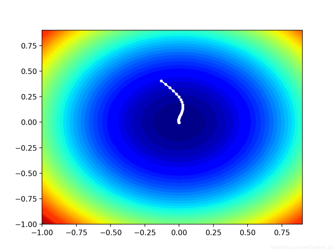
運(yùn)行示例將像以前一樣執(zhí)行搜索,但是在這種情況下,將創(chuàng)建目標(biāo)函數(shù)的輪廓圖。
在這種情況下,我們可以看到在搜索過程中找到的每個(gè)解決方案都顯示一個(gè)白點(diǎn),從最優(yōu)點(diǎn)開始,逐漸靠近圖中心的最優(yōu)點(diǎn)。