近幾年來語音識別技術得到了迅速發展，從手機中的Siri語音智能助手、微軟的小娜以及各種平臺的智能音箱等等，各種語音識別的項目得到了廣泛應用。

語音識別屬于感知智能，而讓機器從簡單的識別語音到理解語音，則上升到了認知智能層面，機器的自然語言理解能力如何，也成為了其是否有智慧的標志，而自然語言理解正是目前難點。

同時考慮到目前大多數的語音識別平臺都是借助于智能云，對于語音識別的訓練對于大多數人而言還較為神秘，故今天我們將利用python搭建自己的語音識別系統。

最終模型的識別效果如下：

[[396315]]

實驗前的準備

首先我們使用的python版本是3.6.5所用到的庫有cv2庫用來圖像處理；

Numpy庫用來矩陣運算；Keras框架用來訓練和加載模型。Librosa和python_speech_features庫用于提取音頻特征。Glob和pickle庫用來讀取本地數據集。

[[396316]]

數據集準備
首先數據集使用的是清華大學的thchs30中文數據。

這些錄音根據其文本內容分成了四部分，A（句子的ID是1~250），B（句子的ID是251~500），C（501~750），D（751~1000）。ABC三組包括30個人的10893句發音，用來做訓練，D包括10個人的2496句發音，用來做測試。

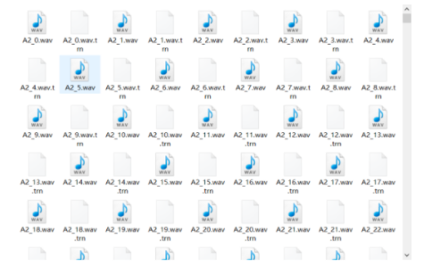
data文件夾中包含（.wav文件和.trn文件；trn文件里存放的是.wav文件的文字描述:第一行為詞，第二行為拼音，第三行為音素）；

數據集如下：

[[396317]]

模型訓練

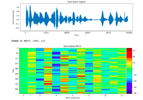
1、提取語音數據集的MFCC特征：
首先人的聲音是通過聲道產生的，聲道的形狀決定了發出怎樣的聲音。如果我們可以準確的知道這個形狀，那么我們就可以對產生的音素進行準確的描述。聲道的形狀在語音短時功率譜的包絡中顯示出來。而MFCCs就是一種準確描述這個包絡的一種特征。

其中提取的MFCC特征如下圖可見。

故我們在讀取數據集的基礎上，要將其語音特征提取存儲以方便加載入神經網絡進行訓練。

其對應的代碼如下：

#讀取數據集文件 
 
text_paths = glob.glob('data/*.trn') 
 
total = len(text_paths) 
 
print(total) 
 
with open(text_paths[0], 'r', encoding='utf8') as fr: 
 
lines = fr.readlines 
 
print(lines) 
 
#數據集文件trn內容讀取保存到數組中 
 
texts =  
 
paths =  
 
for path in text_paths: 
 
with open(path, 'r', encoding='utf8') as fr: 
 
lines = fr.readlines 
 
line = lines[0].strip('\n').replace(' ', '') 
 
texts.append(line) 
 
paths.append(path.rstrip('.trn')) 
 
print(paths[0], texts[0]) 
 
#定義mfcc數 
 
mfcc_dim = 13 
 
#根據數據集標定的音素讀入 
 
def load_and_trim(path): 
 
audio, sr = librosa.load(path) 
 
energy = librosa.feature.rmse(audio) 
 
frames = np.nonzero(energy >= np.max(energy) / 5) 
 
indices = librosa.core.frames_to_samples(frames)[1] 
 
audio = audio[indices[0]:indices[-1]] if indices.size else audio[0:0] 
 
return audio, sr 
 
#提取音頻特征并存儲 
 
features =  
 
for i in tqdm(range(total)): 
 
path = paths[i] 
 
audio, sr = load_and_trim(path) 
 
features.append(mfcc(audio, sr, numcep=mfcc_dim, nfft=551)) 
 
print(len(features), features[0].shape) 

2、神經網絡預處理：
在進行神經網絡加載訓練前，我們需要對讀取的MFCC特征進行歸一化，主要目的是為了加快收斂，提高效果和減少干擾。然后處理好數據集和標簽定義輸入和輸出即可。

對應代碼如下：

#隨機選擇100個數據集 
 
samples = random.sample(features, 100) 
 
samples = np.vstack(samples) 
 
#平均MFCC的值為了歸一化處理 
 
mfcc_mean = np.mean(samples, axis=0) 
 
#計算標準差為了歸一化 
 
mfcc_std = np.std(samples, axis=0) 
 
print(mfcc_mean) 
 
print(mfcc_std) 
 
#歸一化特征 
 
features = [(feature - mfcc_mean) / (mfcc_std + 1e-14) for feature in features] 
 
#將數據集讀入的標簽和對應id存儲列表 
 
chars = {} 
 
for text in texts: 
 
for c in text: 
 
chars[c] = chars.get(c, 0) + 1 
 
chars = sorted(chars.items, key=lambda x: x[1], reverse=True) 
 
chars = [char[0] for char in chars] 
 
print(len(chars), chars[:100]) 
 
char2id = {c: i for i, c in enumerate(chars)} 
 
id2char = {i: c for i, c in enumerate(chars)} 
 
data_index = np.arange(total) 
 
np.random.shuffle(data_index) 
 
train_size = int(0.9 * total) 
 
test_size = total - train_size 
 
train_index = data_index[:train_size] 
 
test_index = data_index[train_size:] 
 
#神經網絡輸入和輸出X,Y的讀入數據集特征 
 
X_train = [features[i] for i in train_index] 
 
Y_train = [texts[i] for i in train_index] 
 
X_test = [features[i] for i in test_index] 
 
Y_test = [texts[i] for i in test_index] 

3、神經網絡函數定義：
其中包括訓練的批次，卷積層函數、標準化函數、激活層函數等等。

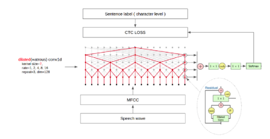
其中第⼀個維度為⼩⽚段的個數，原始語⾳越長，第⼀個維度也越⼤， 第⼆個維度為 MFCC 特征的維度。得到原始語⾳的數值表⽰后，就可以使⽤ WaveNet 實現。由于 MFCC 特征為⼀維序列，所以使⽤ Conv1D 進⾏卷積。 因果是指，卷積的輸出只和當前位置之前的輸⼊有關，即不使⽤未來的 特征，可以理解為將卷積的位置向前偏移。WaveNet 模型結構如下所⽰：

具體如下可見：

batch_size = 16 
 
#定義訓練批次的產生，一次訓練16個 
 
def batch_generator(x, y, batch_size=batch_size): 
 
offset = 0 
 
while True: 
 
offset += batch_size 
 
if offset == batch_size or offset >= len(x): 
 
data_index = np.arange(len(x)) 
 
np.random.shuffle(data_index) 
 
x = [x[i] for i in data_index] 
 
y = [y[i] for i in data_index] 
 
offset = batch_size 
 
X_data = x[offset - batch_size: offset] 
 
Y_data = y[offset - batch_size: offset] 
 
X_maxlen = max([X_data[i].shape[0] for i in range(batch_size)]) 
 
Y_maxlen = max([len(Y_data[i]) for i in range(batch_size)]) 
 
X_batch = np.zeros([batch_size, X_maxlen, mfcc_dim]) 
 
Y_batch = np.ones([batch_size, Y_maxlen]) * len(char2id) 
 
X_length = np.zeros([batch_size, 1], dtype='int32') 
 
Y_length = np.zeros([batch_size, 1], dtype='int32') 
 
for i in range(batch_size): 
 
X_length[i, 0] = X_data[i].shape[0] 
 
X_batch[i, :X_length[i, 0], :] = X_data[i] 
 
Y_length[i, 0] = len(Y_data[i]) 
 
Y_batch[i, :Y_length[i, 0]] = [char2id[c] for c in Y_data[i]] 
 
inputs = {'X': X_batch, 'Y': Y_batch, 'X_length': X_length, 'Y_length': Y_length} 
 
outputs = {'ctc': np.zeros([batch_size])} 
 
epochs = 50 
 
num_blocks = 3 
 
filters = 128 
 
X = Input(shape=(None, mfcc_dim,), dtype='float32', name='X') 
 
Y = Input(shape=(None,), dtype='float32', name='Y') 
 
X_length = Input(shape=(1,), dtype='int32', name='X_length') 
 
Y_length = Input(shape=(1,), dtype='int32', name='Y_length') 
 
#卷積1層 
 
def conv1d(inputs, filters, kernel_size, dilation_rate): 
 
return Conv1D(filters=filters, kernel_size=kernel_size, strides=1, padding='causal', activation=None, 
 
dilation_rate=dilation_rate)(inputs) 
 
#標準化函數 
 
def batchnorm(inputs): 
 
return BatchNormalization(inputs) 
 
#激活層函數 
 
def activation(inputs, activation): 
 
return Activation(activation)(inputs) 
 
#全連接層函數 
 
def res_block(inputs, filters, kernel_size, dilation_rate): 
 
hf = activation(batchnorm(conv1d(inputs, filters, kernel_size, dilation_rate)), 'tanh') 
 
hg = activation(batchnorm(conv1d(inputs, filters, kernel_size, dilation_rate)), 'sigmoid') 
 
h0 = Multiply([hf, hg]) 
 
ha = activation(batchnorm(conv1d(h0, filters, 1, 1)), 'tanh') 
 
hs = activation(batchnorm(conv1d(h0, filters, 1, 1)), 'tanh') 
 
return Add([ha, inputs]), hs 
 
h0 = activation(batchnorm(conv1d(X, filters, 1, 1)), 'tanh') 
 
shortcut =  
 
for i in range(num_blocks): 
 
for r in [1, 2, 4, 8, 16]: 
 
h0, s = res_block(h0, filters, 7, r) 
 
shortcut.append(s) 
 
h1 = activation(Add(shortcut), 'relu') 
 
h1 = activation(batchnorm(conv1d(h1, filters, 1, 1)), 'relu') 
 
#softmax損失函數輸出結果 
 
Y_pred = activation(batchnorm(conv1d(h1, len(char2id) + 1, 1, 1)), 'softmax') 
 
sub_model = Model(inputs=X, outputs=Y_pred) 
 
#計算損失函數 
 
def calc_ctc_loss(args): 
 
y, yp, ypl, yl = args 
 
return K.ctc_batch_cost(y, yp, ypl, yl) 

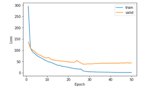
4、模型的訓練：
訓練的過程如下可見：

ctc_loss = Lambda(calc_ctc_loss, output_shape=(1,), name='ctc')([Y, Y_pred, X_length, Y_length]) 
 
#加載模型訓練 
 
model = Model(inputs=[X, Y, X_length, Y_length], outputs=ctc_loss) 
 
#建立優化器 
 
optimizer = SGD(lr=0.02, momentum=0.9, nesterov=True, clipnorm=5) 
 
#激活模型開始計算 
 
model.compile(loss={'ctc': lambda ctc_true, ctc_pred: ctc_pred}, optimizer=optimizer) 
 
checkpointer = ModelCheckpoint(filepath='asr.h5', verbose=0) 
 
lr_decay = ReduceLROnPlateau(monitor='loss', factor=0.2, patience=1, min_lr=0.000) 
 
#開始訓練 
 
history = model.fit_generator( 
 
generator=batch_generator(X_train, Y_train), 
 
steps_per_epoch=len(X_train) // batch_size, 
 
epochs=epochs, 
 
validation_data=batch_generator(X_test, Y_test), 
 
validation_steps=len(X_test) // batch_size, 
 
callbacks=[checkpointer, lr_decay]) 
 
#保存模型 
 
sub_model.save('asr.h5') 
 
#將字保存在pl=pkl中 
 
with open('dictionary.pkl', 'wb') as fw: 
 
pickle.dump([char2id, id2char, mfcc_mean, mfcc_std], fw) 
 
train_loss = history.history['loss'] 
 
valid_loss = history.history['val_loss'] 
 
plt.plot(np.linspace(1, epochs, epochs), train_loss, label='train') 
 
plt.plot(np.linspace(1, epochs, epochs), valid_loss, label='valid') 
 
plt.legend(loc='upper right') 
 
plt.xlabel('Epoch') 
 
plt.ylabel('Loss') 
 
plt.show 

[[396319]]

測試模型
讀取我們語音數據集生成的字典，通過調用模型來對音頻特征識別。

代碼如下：

wavs = glob.glob('A2_103.wav') 
 
print(wavs) 
 
with open('dictionary.pkl', 'rb') as fr: 
 
[char2id, id2char, mfcc_mean, mfcc_std] = pickle.load(fr) 
 
mfcc_dim = 13 
 
model = load_model('asr.h5') 
 
index = np.random.randint(len(wavs)) 
 
print(wavs[index]) 
 
audio, sr = librosa.load(wavs[index]) 
 
energy = librosa.feature.rmse(audio) 
 
frames = np.nonzero(energy >= np.max(energy) / 5) 
 
indices = librosa.core.frames_to_samples(frames)[1] 
 
audio = audio[indices[0]:indices[-1]] if indices.size else audio[0:0] 
 
X_data = mfcc(audio, sr, numcep=mfcc_dim, nfft=551) 
 
X_data = (X_data - mfcc_mean) / (mfcc_std + 1e-14) 
 
print(X_data.shape) 
 
pred = model.predict(np.expand_dims(X_data, axis=0)) 
 
pred_ids = K.eval(K.ctc_decode(pred, [X_data.shape[0]], greedy=False, beam_width=10, top_paths=1)[0][0]) 
 
pred_ids = pred_ids.flatten.tolist 
 
print(''.join([id2char[i] for i in pred_ids])) 
 
yield (inputs, outputs) 

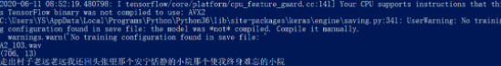
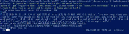
到這里，我們整體的程序就搭建完成，下面為我們程序的運行結果：

源碼地址：

https://pan.baidu.com/s/1tFlZkMJmrMTD05cd_zxmAg

提取碼：ndrr

數據集需要自行下載。