[[387235]]

爬坡測試集是一種在不影響訓練集甚至開發預測模型的情況下，在機器學習競賽中實現良好或完美預測的方法。作為機器學習競賽的一種方法，這是理所當然的，大多數競賽平臺都對其施加了限制，以防止出現這種情況，這一點很重要。但是，爬坡測試集是機器學習從業人員在參加比賽時不小心做的事情。通過開發一個明確的實現來爬升測試集，它有助于更好地了解通過過度使用測試數據集來評估建模管道而過度擬合測試數據集的難易程度。

在本教程中，您將發現如何爬升用于機器學習的測試集。完成本教程后，您將知道：

•  無需查看訓練數據集，就可以通過爬上測試集來做出完美的預測。
•  如何為分類和回歸任務爬坡測試集。
•  當我們過度使用測試集來評估建模管道時，我們暗中爬升了測試集。

教程概述

本教程分為五個部分。他們是：

•  爬坡測試儀
•  爬山算法
•  如何進行爬山
•  爬坡糖尿病分類數據集
•  爬坡房屋回歸數據集

爬坡測試儀

像Kaggle上的機器學習比賽一樣，機器學習比賽提供了完整的訓練數據集以及測試集的輸入。給定比賽的目的是預測目標值，例如測試集的標簽或數值。針對隱藏的測試設置目標值評估解決方案，并進行適當評分。與測試集得分最高的參賽作品贏得了比賽。機器學習競賽的挑戰可以被定義為一個優化問題。傳統上，競賽參與者充當優化算法，探索導致不同組預測的不同建模管道，對預測進行評分，然后對管道進行更改以期望獲得更高的分數。此過程也可以直接用優化算法建模，無需查看訓練集就可以生成和評估候選預測。通常，這稱為爬山測試集，作為解決此問題的最簡單的優化算法之一就是爬山算法。盡管在實際的機器學習競賽中應該正確地爬升測試集，但是實施該方法以了解該方法的局限性和過度安裝測試集的危險可能是一個有趣的練習。此外，無需接觸訓練數據集就可以完美預測測試集的事實常常使很多初學者機器學習從業人員感到震驚。最重要的是，當我們反復評估不同的建模管道時，我們暗中爬升了測試集。風險是測試集的分數得到了提高，但代價是泛化誤差增加，即在更廣泛的問題上表現較差。進行機器學習競賽的人們都非常清楚這個問題，并且對預測評估施加了限制以應對該問題，例如將評估限制為每天一次或幾次，并在測試集的隱藏子集而不是整個測試集上報告分數。。有關更多信息，請參閱進一步閱讀部分中列出的論文。接下來，讓我們看看如何實施爬坡算法來優化測試集的預測。

爬山算法

爬山算法是一種非常簡單的優化算法。它涉及生成候選解決方案并進行評估。然后是逐步改進的起點，直到無法實現進一步的改進，或者我們用光了時間，資源或興趣。從現有候選解決方案中生成新的候選解決方案。通常，這涉及對候選解決方案進行單個更改，對其進行評估，并且如果候選解決方案與先前的當前解決方案一樣好或更好，則將該候選解決方案接受為新的“當前”解決方案。否則，將其丟棄。我們可能會認為只接受分數更高的候選人是一個好主意。對于許多簡單問題，這是一種合理的方法，盡管在更復雜的問題上，希望接受具有相同分數的不同候選者，以幫助搜索過程縮放要素空間中的平坦區域（高原）。當爬上測試集時，候選解決方案是預測列表。對于二進制分類任務，這是兩個類的0和1值的列表。對于回歸任務，這是目標變量范圍內的數字列表。對候選分類解決方案的修改將是選擇一個預測并將其從0翻轉為1或從1翻轉為0。對回歸進行候選解決方案的修改將是將高斯噪聲添加到列表中的一個值或替換一個值在列表中使用新值。解決方案的評分涉及計算評分指標，例如分類任務的分類準確性或回歸任務的平均絕對誤差。現在我們已經熟悉了算法，現在就來實現它。

如何進行爬山

我們將在綜合分類任務上開發爬坡算法。首先，我們創建一個包含許多輸入變量和5,000行示例的二進制分類任務。然后，我們可以將數據集分為訓練集和測試集。下面列出了完整的示例。 

# example of a synthetic dataset.  
from sklearn.datasets import make_classification  
from sklearn.model_selection import train_test_split  
# define dataset  
X, y = make_classification(n_samples=5000, n_features=20, n_informative=15, n_redundant=5, random_state=1)  
print(X.shape, y.shape)  
# split dataset  
X_train, X_test, y_train, y_test = train_test_split(X, y, test_size=0.33, random_state=1) 
print(X_train.shape, X_test.shape, y_train.shape, y_test.shape) 

運行示例首先報告創建的數據集的形狀，顯示5,000行和20個輸入變量。然后將數據集分為訓練集和測試集，其中約3,300個用于訓練，約1,600個用于測試。 

(5000, 20) (5000,)  
(3350, 20) (1650, 20) (3350,) (1650,) 

現在我們可以開發一個登山者。首先，我們可以創建一個將加載的函數，或者在這種情況下，定義數據集。當我們要更改數據集時，可以稍后更新此功能。 

# load or prepare the classification dataset  
def load_dataset():  
 return make_classification(n_samples=5000, n_features=20, n_informative=15, n_redundant=5, random_state=1) 

接下來，我們需要一個函數來評估候選解決方案，即預測列表。我們將使用分類精度，其中分數范圍在0（最壞的解決方案）到1（完美的預測集）之間。 

# evaluate a set of predictions  
def evaluate_predictions(y_test, yhat):  
 return accuracy_score(y_test, yhat) 

接下來，我們需要一個函數來創建初始候選解決方案。這是0和1類標簽的預測列表，長度足以匹配測試集中的示例數，在這種情況下為1650。我們可以使用randint（）函數生成0和1的隨機值。 

# create a random set of predictions  
def random_predictions(n_examples):  
 return [randint(0, 1) for _ in range(n_examples)] 

接下來，我們需要一個函數來創建候選解決方案的修改版本。在這種情況下，這涉及在解決方案中選擇一個值并將其從0翻轉為1或從1翻轉為0。通常，我們會在爬坡期間對每個新的候選解決方案進行一次更改，但是我已經對該函數進行了參數化，因此您可以根據需要探索多個更改。 

# modify the current set of predictions  
def modify_predictions(current, n_changes=1):  
 # copy current solution  
 updated = current.copy() 
 for i in range(n_changes):  
  # select a point to change  
  ix = randint(0, len(updated)-1)  
  # flip the class label  
  updated[ix] = 1 - updated[ix]  
 return updated 

到現在為止還挺好。接下來，我們可以開發執行搜索的功能。首先，通過調用random_predictions（）函數和隨后的validate_predictions（）函數來創建和評估初始解決方案。然后，我們循環進行固定次數的迭代，并通過調用Modify_predictions（）生成一個新的候選值，對其進行求值，如果分數與當前解決方案相同或更好，則將其替換。當我們完成預設的迭代次數（任意選擇）或達到理想分數時，該循環結束，在這種情況下，我們知道其精度為1.0（100％）。下面的函數hill_climb_testset（）實現了此功能，將測試集作為輸入并返回在爬坡過程中發現的最佳預測集。 

# run a hill climb for a set of predictions  
def hill_climb_testset(X_test, y_test, max_iterations):  
 scores = list()  
 # generate the initial solution  
 solution = random_predictions(X_test.shape[0])  
 # evaluate the initial solution  
 score = evaluate_predictions(y_test, solution) 
 scores.append(score)  
 # hill climb to a solution  
 for i in range(max_iterations):  
  # record scores  
  scores.append(score)  
  # stop once we achieve the best score  
  if score == 1.0:  
   break  
  # generate new candidate  
  candidate = modify_predictions(solution)  
  # evaluate candidate  
  value = evaluate_predictions(y_test, candidate)  
  # check if it is as good or better  
  if value >= score:  
   solution, score = candidate, value  
   print('>%d, score=%.3f' % (i, score))  
 return solution, scores 

這里的所有都是它的。下面列出了爬坡測試裝置的完整示例。 

# example of hill climbing the test set for a classification task  
from random import randint  
from sklearn.datasets import make_classification  
from sklearn.model_selection import train_test_split 
from sklearn.metrics import accuracy_score  
from matplotlib import pyplot   
# load or prepare the classification dataset  
def load_dataset():  
 return make_classification(n_samples=5000, n_features=20, n_informative=15, n_redundant=5, random_state=1)   
# evaluate a set of predictions  
def evaluate_predictions(y_test, yhat):  
 return accuracy_score(y_test, yhat)   
# create a random set of predictions  
def random_predictions(n_examples):  
 return [randint(0, 1) for _ in range(n_examples)] 
# modify the current set of predictions  
def modify_predictions(current, n_changes=1):  
 # copy current solution  
 updated = current.copy()  
 for i in range(n_changes):  
  # select a point to change  
  ix = randint(0, len(updated)-1)  
  # flip the class label  
  updated[ix] = 1 - updated[ix]  
 return updated   
# run a hill climb for a set of predictions  
def hill_climb_testset(X_test, y_test, max_iterations):  
 scores = list()  
 # generate the initial solution  
 solution = random_predictions(X_test.shape[0])  
 # evaluate the initial solution  
 score = evaluate_predictions(y_test, solution)  
 scores.append(score)  
 # hill climb to a solution  
 for i in range(max_iterations):  
  # record scores  
  scores.append(score)  
  # stop once we achieve the best score  
  if score == 1.0:  
   break  
  # generate new candidate  
  candidate = modify_predictions(solution)  
  # evaluate candidate  
  value = evaluate_predictions(y_test, candidate)  
  # check if it is as good or better  
  if value >= score:  
   solution, score = candidate, value  
   print('>%d, score=%.3f' % (i, score))  
 return solution, scores  
# load the dataset  
X, y = load_dataset()  
print(X.shape, y.shape)  
# split dataset into train and test sets  
X_train, X_test, y_train, y_test = train_test_split(X, y, test_size=0.33, random_state=1)  
print(X_train.shape, X_test.shape, y_train.shape, y_test.shape)  
# run hill climb  
yhat, scores = hill_climb_testset(X_test, y_test, 20000)  
# plot the scores vs iterations 
pyplot.plot(scores)  
pyplot.show() 

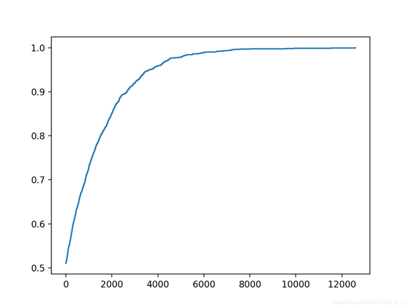
運行示例將使搜索進行20,000次迭代，或者如果達到理想的準確性，則停止搜索。注意：由于算法或評估程序的隨機性，或者數值精度的差異，您的結果可能會有所不同。考慮運行該示例幾次并比較平均結果。在這種情況下，我們在約12,900次迭代中找到了一組理想的測試集預測。回想一下，這是在不接觸訓練數據集且不通過查看測試集目標值進行欺騙的情況下實現的。相反，我們只是簡單地優化了一組數字。這里的教訓是，將測試管道用作爬山優化算法，對測試集重復建模管道的評估會做同樣的事情。解決方案將過度適合測試集。 

...  
>8092, score=0.996  
>8886, score=0.997  
>9202, score=0.998  
>9322, score=0.998  
>9521, score=0.999  
>11046, score=0.999  
>12932, score=1.000 

還創建了優化進度圖。這有助于了解優化算法的更改（例如，在坡道上更改內容的選擇以及更改方式）如何影響搜索的收斂性。

爬坡糖尿病分類數據集

我們將使用糖尿病數據集作為探索爬坡測試集以解決分類問題的基礎。每條記錄都描述了女性的醫療細節，并且預測是未來五年內糖尿病的發作。

數據集詳細信息：pima-indians-diabetes.names數據集：pima-indians-diabetes.csv

數據集有八個輸入變量和768行數據；輸入變量均為數字，目標具有兩個類別標簽，例如 這是一個二進制分類任務。下面提供了數據集前五行的示例。 

6,148,72,35,0,33.6,0.627,50,1  
1,85,66,29,0,26.6,0.351,31,0  
8,183,64,0,0,23.3,0.672,32,1  
1,89,66,23,94,28.1,0.167,21,0  
0,137,40,35,168,43.1,2.288,33,1  
... 

我們可以使用Pandas直接加載數據集，如下所示。 

# load or prepare the classification dataset  
def load_dataset(): 
  url = 'https://raw.githubusercontent.com/jbrownlee/Datasets/master/pima-indians-diabetes.csv'  
 df = read_csv(url, header=None) 
 data = df.values  
 return data[:, :-1], data[:, -1] 

其余代碼保持不變。創建該文件是為了使您可以放入自己的二進制分類任務并進行嘗試。下面列出了完整的示例。 

# example of hill climbing the test set for the diabetes dataset  
from random import randint  
from pandas import read_csv  
from sklearn.model_selection import train_test_split  
from sklearn.metrics import accuracy_score  
from matplotlib import pyplot   
# load or prepare the classification dataset  
def load_dataset():  
 url = 'https://raw.githubusercontent.com/jbrownlee/Datasets/master/pima-indians-diabetes.csv'  
 df = read_csv(url, header=None)  
 data = df.values  
 return data[:, :-1], data[:, -1]  
# evaluate a set of predictions  
def evaluate_predictions(y_test, yhat):  
 return accuracy_score(y_test, yhat)   
# create a random set of predictions  
def random_predictions(n_examples):  
 return [randint(0, 1) for _ in range(n_examples)]  
# modify the current set of predictions  
def modify_predictions(current, n_changes=1):  
 # copy current solution  
 updated = current.copy()  
 for i in range(n_changes):  
  # select a point to change  
  ix = randint(0, len(updated)-1)  
  # flip the class label  
  updated[ix] = 1 - updated[ix]  
 return updated   
# run a hill climb for a set of predictions  
def hill_climb_testset(X_test, y_test, max_iterations):  
 scores = list()  
 # generate the initial solution  
 solution = random_predictions(X_test.shape[0])  
 # evaluate the initial solution  
 score = evaluate_predictions(y_test, solution)  
 scores.append(score)  
 # hill climb to a solution  
 for i in range(max_iterations):  
  # record scores  
  scores.append(score)  
  # stop once we achieve the best score  
  if score == 1.0: 
   break  
  # generate new candidate  
  candidate = modify_predictions(solution)  
  # evaluate candidate  
  value = evaluate_predictions(y_test, candidate)  
  # check if it is as good or better  
  if value >= score:  
   solution, score = candidate, value  
   print('>%d, score=%.3f' % (i, score))  
 return solution, scores  
# load the dataset  
X, y = load_dataset()  
print(X.shape, y.shape)  
# split dataset into train and test sets  
X_train, X_test, y_train, y_test = train_test_split(X, y, test_size=0.33, random_state=1)  
print(X_train.shape, X_test.shape, y_train.shape, y_test.shape)  
# run hill climb  
yhat, scores = hill_climb_testset(X_test, y_test, 5000)  
# plot the scores vs iterations  
pyplot.plot(scores)  
pyplot.show() 

運行示例將報告每次搜索過程中看到改進時的迭代次數和準確性。

在這種情況下，我們使用的迭代次數較少，因為要進行的預測較少，因此優化起來比較簡單。

注意：由于算法或評估程序的隨機性，或者數值精度的差異，您的結果可能會有所不同。考慮運行該示例幾次并比較平均結果。

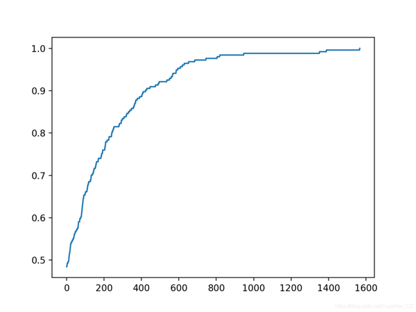
在這種情況下，我們可以看到在大約1,500次迭代中達到了完美的精度。 

...  
>617, score=0.961  
>627, score=0.965  
>650, score=0.969  
>683, score=0.972  
>743, score=0.976  
>803, score=0.980  
>817, score=0.984  
>945, score=0.988  
>1350, score=0.992  
>1387, score=0.996  
>1565, score=1.000 

還創建了搜索進度的折線圖，表明收斂迅速。

爬坡房屋回歸數據集

我們將使用住房數據集作為探索爬坡測試集回歸問題的基礎。住房數據集包含給定房屋及其附近地區詳細信息的數千美元房屋價格預測。

數據集詳細信息：housing.names數據集：housing.csv

這是一個回歸問題，這意味著我們正在預測一個數值。共有506個觀測值，其中包含13個輸入變量和一個輸出變量。下面列出了前五行的示例。 

0.00632,18.00,2.310,0,0.5380,6.5750,65.20,4.0900,1,296.0,15.30,396.90,4.98,24.00  
0.02731,0.00,7.070,0,0.4690,6.4210,78.90,4.9671,2,242.0,17.80,396.90,9.14,21.60 
0.02729,0.00,7.070,0,0.4690,7.1850,61.10,4.9671,2,242.0,17.80,392.83,4.03,34.70  
0.03237,0.00,2.180,0,0.4580,6.9980,45.80,6.0622,3,222.0,18.70,394.63,2.94,33.40  
0.06905,0.00,2.180,0,0.4580,7.1470,54.20,6.0622,3,222.0,18.70,396.90,5.33,36.20 
 ... 

首先，我們可以更新load_dataset（）函數以加載住房數據集。作為加載數據集的一部分，我們將標準化目標值。由于我們可以將浮點值限制在0到1的范圍內，這將使爬坡的預測更加簡單。通常不需要這樣做，只是此處采用的簡化搜索算法的方法。 

# load or prepare the classification dataset  
def load_dataset():  
 url = 'https://raw.githubusercontent.com/jbrownlee/Datasets/master/housing.csv'  
 df = read_csv(url, header=None)  
 data = df.values  
 X, y = data[:, :-1], data[:, -1]  
 # normalize the target  
 scaler = MinMaxScaler()  
 yy = y.reshape((len(y), 1))  
 y = scaler.fit_transform(y)  
 return X, y 

接下來，我們可以更新評分函數，以使用預期值和預測值之間的平均絕對誤差。 

# evaluate a set of predictions  
def evaluate_predictions(y_test, yhat):  
 return mean_absolute_error(y_test, yhat) 

我們還必須將解決方案的表示形式從0和1標簽更新為介于0和1之間的浮點值。必須更改初始候選解的生成以創建隨機浮點列表。 

# create a random set of predictions  
def random_predictions(n_examples):  
 return [random() for _ in range(n_examples)] 

在這種情況下，對解決方案所做的單個更改以創建新的候選解決方案，包括簡單地用新的隨機浮點數替換列表中的隨機選擇的預測。我選擇它是因為它很簡單。 

# modify the current set of predictions  
def modify_predictions(current, n_changes=1):  
 # copy current solution  
 updated = current.copy()  
 for i in range(n_changes):  
  # select a point to change  
  ix = randint(0, len(updated)-1)  
  # flip the class label  
  updated[ix] = random()  
 return updated 

更好的方法是將高斯噪聲添加到現有值，我將其作為擴展留給您。如果您嘗試過，請在下面的評論中告訴我。例如： 

# add gaussian noise  
updated[ix] += gauss(0, 0.1) 

最后，必須更新搜索。最佳值現在是錯誤0.0，如果發現錯誤，該錯誤將用于停止搜索。 

# stop once we achieve the best score  
if score == 0.0:  
 break 

我們還需要將搜索從最大分數更改為現在最小分數。 

# check if it is as good or better  
if value <= score:  
 solution, score = candidate, value  
 print('>%d, score=%.3f' % (i, score)) 

下面列出了具有這兩個更改的更新的搜索功能。 

# run a hill climb for a set of predictions  
def hill_climb_testset(X_test, y_test, max_iterations):  
 scores = list()  
 # generate the initial solution  
 solution = random_predictions(X_test.shape[0])  
 # evaluate the initial solution  
 score = evaluate_predictions(y_test, solution)  
 print('>%.3f' % score)  
 # hill climb to a solution  
 for i in range(max_iterations):  
  # record scores  
  scores.append(score)  
  # stop once we achieve the best score  
  if score == 0.0:  
   break  
  # generate new candidate  
  candidate = modify_predictions(solution)  
  # evaluate candidate  
  value = evaluate_predictions(y_test, candidate)  
  # check if it is as good or better  
  if value <= score:  
   solution, score = candidate, value  
   print('>%d, score=%.3f' % (i, score))  
 return solution, scores 

結合在一起，下面列出了用于回歸任務的測試集爬坡的完整示例。 

# example of hill climbing the test set for the housing dataset  
from random import random  
from random import randint  
from pandas import read_csv  
from sklearn.model_selection import train_test_split  
from sklearn.metrics import mean_absolute_error  
from sklearn.preprocessing import MinMaxScaler  
from matplotlib import pyplot   
# load or prepare the classification dataset 
def load_dataset():  
 url = 'https://raw.githubusercontent.com/jbrownlee/Datasets/master/housing.csv'  
 df = read_csv(url, header=None)  
 data = df.values  
 X, y = data[:, :-1], data[:, -1]  
 # normalize the target  
 scaler = MinMaxScaler()  
 yy = y.reshape((len(y), 1))  
 y = scaler.fit_transform(y)  
 return X, y  
# evaluate a set of predictions  
def evaluate_predictions(y_test, yhat):  
 return mean_absolute_error(y_test, yhat)   
# create a random set of predictions  
def random_predictions(n_examples): 
  return [random() for _ in range(n_examples)]  
# modify the current set of predictions  
def modify_predictions(current, n_changes=1):  
 # copy current solution  
 updated = current.copy()  
 for i in range(n_changes):  
  # select a point to change  
  ix = randint(0, len(updated)-1)  
  # flip the class label  
  updated[ix] = random()  
 return updated   
# run a hill climb for a set of predictions  
def hill_climb_testset(X_test, y_test, max_iterations):  
 scores = list()  
 # generate the initial solution  
 solution = random_predictions(X_test.shape[0])  
 # evaluate the initial solution  
 score = evaluate_predictions(y_test, solution)  
 print('>%.3f' % score)  
 # hill climb to a solution  
 for i in range(max_iterations):  
  # record scores  
  scores.append(score)  
  # stop once we achieve the best score  
  if score == 0.0:  
   break  
  # generate new candidate  
  candidate = modify_predictions(solution)  
  # evaluate candidate  
  value = evaluate_predictions(y_test, candidate)  
  # check if it is as good or better  
  if value <= score:  
   solution, score = candidate, value  
   print('>%d, score=%.3f' % (i, score))  
 return solution, scores  
# load the dataset  
X, y = load_dataset()  
print(X.shape, y.shape)  
# split dataset into train and test sets  
X_train, X_test, y_train, y_test = train_test_split(X, y, test_size=0.33, random_state=1)  
print(X_train.shape, X_test.shape, y_train.shape, y_test.shape)  
# run hill climb  
yhat, scores = hill_climb_testset(X_test, y_test, 100000)  
# plot the scores vs iterations  
pyplot.plot(scores)  
pyplot.show() 

運行示例將在搜索過程中每次看到改進時報告迭代次數和MAE。

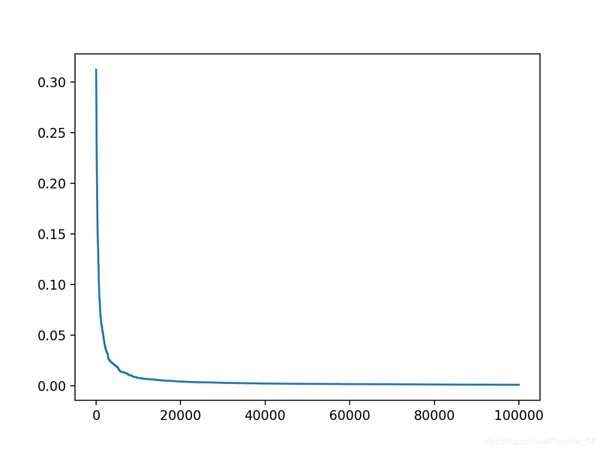
在這種情況下，我們將使用更多的迭代，因為要優化它是一個更復雜的問題。選擇的用于創建候選解決方案的方法也使它變慢了，也不太可能實現完美的誤差。實際上，我們不會實現完美的錯誤；相反，如果錯誤達到的值低于最小值（例如1e-7）或對目標域有意義的值，則最好停止操作。這也留給讀者作為練習。例如： 

# stop once we achieve a good enough  
if score <= 1e-7:  
 break 

注意：由于算法或評估程序的隨機性，或者數值精度的差異，您的結果可能會有所不同。考慮運行該示例幾次并比較平均結果。

在這種情況下，我們可以看到在運行結束時實現了良好的錯誤。 

>95991, score=0.001  
>96011, score=0.001  
>96295, score=0.001  
>96366, score=0.001  
>96585, score=0.001  
>97575, score=0.001  
>98828, score=0.001  
>98947, score=0.001  
>99712, score=0.001  
>99913, score=0.001 

還創建了搜索進度的折線圖，顯示收斂速度很快，并且在大多數迭代中保持不變。