[[405478]]

在本教程中，我們將使用 TensorFlow (Keras API) 實現一個用于多分類任務的深度學習模型，該任務需要對阿拉伯語手寫字符數據集進行識別。

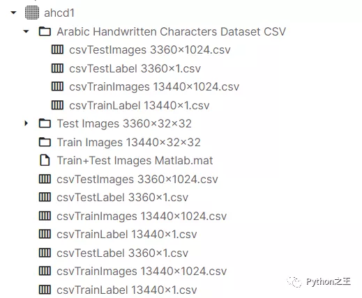
數據集下載地址：https://www.kaggle.com/mloey1/ahcd1

數據集介紹

該數據集由 60 名參與者書寫的16,800 個字符組成，年齡范圍在 19 至 40 歲之間，90% 的參與者是右手。

每個參與者在兩種形式上寫下每個字符(從“alef”到“yeh”)十次，如圖 7(a)和 7(b)所示。表格以 300 dpi 的分辨率掃描。使用 Matlab 2016a 自動分割每個塊以確定每個塊的坐標。該數據庫分為兩組：訓練集(每類 13,440 個字符到 480 個圖像)和測試集(每類 3,360 個字符到 120 個圖像)。數據標簽為1到28個類別。在這里，所有數據集都是CSV文件，表示圖像像素值及其相應標簽，并沒有提供對應的圖片數據。

導入模塊

import numpy as np 
import pandas as pd 
#允許對dataframe使用display（） 
from IPython.display import display 
# 導入讀取和處理圖像所需的庫 
import csv 
from PIL import Image 
from scipy.ndimage import rotate 

讀取數據

# 訓練數據images 
letters_training_images_file_path = "../input/ahcd1/csvTrainImages 13440x1024.csv" 
# 訓練數據labels 
letters_training_labels_file_path = "../input/ahcd1/csvTrainLabel 13440x1.csv" 
# 測試數據images和labels 
letters_testing_images_file_path = "../input/ahcd1/csvTestImages 3360x1024.csv" 
letters_testing_labels_file_path = "../input/ahcd1/csvTestLabel 3360x1.csv" 
 
# 加載數據 
training_letters_images = pd.read_csv(letters_training_images_file_path, header=None) 
training_letters_labels = pd.read_csv(letters_training_labels_file_path, header=None) 
testing_letters_images = pd.read_csv(letters_testing_images_file_path, header=None) 
testing_letters_labels = pd.read_csv(letters_testing_labels_file_path, header=None) 
 
print("%d個32x32像素的訓練阿拉伯字母圖像。" %training_letters_images.shape[0]) 
print("%d個32x32像素的測試阿拉伯字母圖像。" %testing_letters_images.shape[0]) 
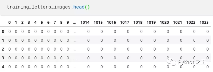
training_letters_images.head() 

13440個32x32像素的訓練阿拉伯字母圖像。3360個32x32像素的測試阿拉伯字母圖像。

查看訓練數據的head

np.unique(training_letters_labels) 
array([ 1,  2,  3,  4,  5,  6,  7,  8,  9, 10, 11, 12, 13, 14, 15, 16, 17,18, 19, 20, 21, 22, 23, 24, 25, 26, 27, 28], dtype=int32) 

下面需要將csv值轉換為圖像，我們希望展示對應圖像的像素值圖像。

def convert_values_to_image(image_values, display=False): 
    image_array = np.asarray(image_values) 
    image_array = image_array.reshape(32,32).astype('uint8') 
    # 原始數據集被反射，因此我們將使用np.flip翻轉它，然后通過rotate旋轉，以獲得更好的圖像。 
    image_array = np.flip(image_array, 0) 
    image_array = rotate(image_array, -90) 
    new_image = Image.fromarray(image_array) 
    if display == True: 
        new_image.show() 
    return new_image 
convert_values_to_image(training_letters_images.loc[0], True) 

 這是一個字母f。

下面，我們將進行數據預處理，主要進行圖像標準化，我們通過將圖像中的每個像素除以255來重新縮放圖像，標準化到[0，1]

training_letters_images_scaled = training_letters_images.values.astype('float32')/255 
training_letters_labels = training_letters_labels.values.astype('int32') 
testing_letters_images_scaled = testing_letters_images.values.astype('float32')/255 
testing_letters_labels = testing_letters_labels.values.astype('int32') 
print("Training images of letters after scaling") 
print(training_letters_images_scaled.shape) 
training_letters_images_scaled[0:5] 

輸出如下

Training images of letters after scaling 
(13440, 1024) 

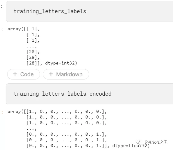
從標簽csv文件我們可以看到，這是一個多類分類問題。下一步需要進行分類標簽編碼，建議將類別向量轉換為矩陣類型。

輸出形式如下：將1到28，變成0到27類別。從“alef”到“yeh”的字母有0到27的分類號。to_categorical就是將類別向量轉換為二進制(只有0和1)的矩陣類型表示

在這里，我們將使用keras的一個熱編碼對這些類別值進行編碼。

一個熱編碼將整數轉換為二進制矩陣，其中數組僅包含一個“1”，其余元素為“0”。

from keras.utils import to_categorical 
 
# one hot encoding 
number_of_classes = 28 
 
training_letters_labels_encoded = to_categorical(training_letters_labels-1, num_classes=number_of_classes) 
testing_letters_labels_encoded = to_categorical(testing_letters_labels-1, num_classes=number_of_classes) 

# (13440, 1024) 

下面將輸入圖像重塑為32x32x1，因為當使用TensorFlow作為后端時，Keras CNN需要一個4D數組作為輸入，并帶有形狀(nb_samples、行、列、通道)

其中 nb_samples對應于圖像(或樣本)的總數，而行、列和通道分別對應于每個圖像的行、列和通道的數量。

# reshape input letter images to 32x32x1 
training_letters_images_scaled = training_letters_images_scaled.reshape([-1, 32, 32, 1]) 
testing_letters_images_scaled = testing_letters_images_scaled.reshape([-1, 32, 32, 1]) 
 
print(training_letters_images_scaled.shape, training_letters_labels_encoded.shape, testing_letters_images_scaled.shape, testing_letters_labels_encoded.shape) 
# (13440, 32, 32, 1) (13440, 28) (3360, 32, 32, 1) (3360, 28) 

因此，我們將把輸入圖像重塑成4D張量形狀(nb_samples，32，32，1)，因為我們圖像是32x32像素的灰度圖像。

#將輸入字母圖像重塑為32x32x1 
training_letters_images_scaled = training_letters_images_scaled.reshape([-1, 32, 32, 1]) 
testing_letters_images_scaled = testing_letters_images_scaled.reshape([-1, 32, 32, 1]) 
 
print(training_letters_images_scaled.shape, training_letters_labels_encoded.shape, testing_letters_images_scaled.shape, testing_letters_labels_encoded.shape) 

設計模型結構

from keras.models import Sequential 
from keras.layers import Conv2D, MaxPooling2D, GlobalAveragePooling2D, BatchNormalization, Dropout, Dense 
 
def create_model(optimizer='adam', kernel_initializer='he_normal', activation='relu'): 
    # create model 
    model = Sequential() 
    model.add(Conv2D(filters=16, kernel_size=3, padding='same', input_shape=(32, 32, 1), kernel_initializer=kernel_initializer, activation=activation)) 
    model.add(BatchNormalization()) 
    model.add(MaxPooling2D(pool_size=2)) 
    model.add(Dropout(0.2)) 
 
    model.add(Conv2D(filters=32, kernel_size=3, padding='same', kernel_initializer=kernel_initializer, activation=activation)) 
    model.add(BatchNormalization()) 
    model.add(MaxPooling2D(pool_size=2)) 
    model.add(Dropout(0.2)) 
 
    model.add(Conv2D(filters=64, kernel_size=3, padding='same', kernel_initializer=kernel_initializer, activation=activation)) 
    model.add(BatchNormalization()) 
    model.add(MaxPooling2D(pool_size=2)) 
    model.add(Dropout(0.2)) 
 
    model.add(Conv2D(filters=128, kernel_size=3, padding='same', kernel_initializer=kernel_initializer, activation=activation)) 
    model.add(BatchNormalization()) 
    model.add(MaxPooling2D(pool_size=2)) 
    model.add(Dropout(0.2)) 
    model.add(GlobalAveragePooling2D()) 
 
    #Fully connected final layer 
    model.add(Dense(28, activation='softmax')) 
 
    # Compile model 
    model.compile(loss='categorical_crossentropy', metrics=['accuracy'], optimizer=optimizer) 
    return model 

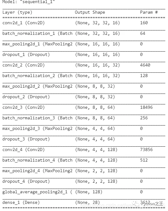
「模型結構」

• 第一隱藏層是卷積層。該層有16個特征圖，大小為3×3和一個激活函數，它是relu。這是輸入層，需要具有上述結構的圖像。
• 第二層是批量標準化層，它解決了特征分布在訓練和測試數據中的變化，BN層添加在激活函數前，對輸入激活函數的輸入進行歸一化。這樣解決了輸入數據發生偏移和增大的影響。
• 第三層是MaxPooling層。最大池層用于對輸入進行下采樣，使模型能夠對特征進行假設，從而減少過擬合。它還減少了參數的學習次數，減少了訓練時間。
• 下一層是使用dropout的正則化層。它被配置為隨機排除層中20%的神經元，以減少過度擬合。
• 另一個隱藏層包含32個要素，大小為3×3和relu激活功能，從圖像中捕捉更多特征。
• 其他隱藏層包含64和128個要素，大小為3×3和一個relu激活功能，
• 重復三次卷積層、MaxPooling、批處理規范化、正則化和* GlobalAveragePooling2D層。
• 最后一層是具有(輸出類數)的輸出層，它使用softmax激活函數，因為我們有多個類。每個神經元將給出該類的概率。
• 使用分類交叉熵作為損失函數，因為它是一個多類分類問題。使用精確度作為衡量標準來提高神經網絡的性能。

model = create_model(optimizer='Adam', kernel_initializer='uniform', activation='relu') 
model.summary() 

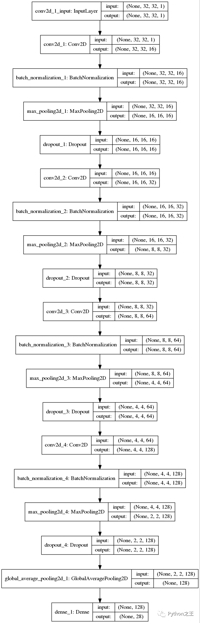
「Keras支持在Keras.utils.vis_utils模塊中繪制模型，該模塊提供了使用graphviz繪制Keras模型的實用函數」

import pydot 
from keras.utils import plot_model 
 
plot_model(model, to_file="model.png", show_shapes=True) 
from IPython.display import Image as IPythonImage 
display(IPythonImage('model.png')) 

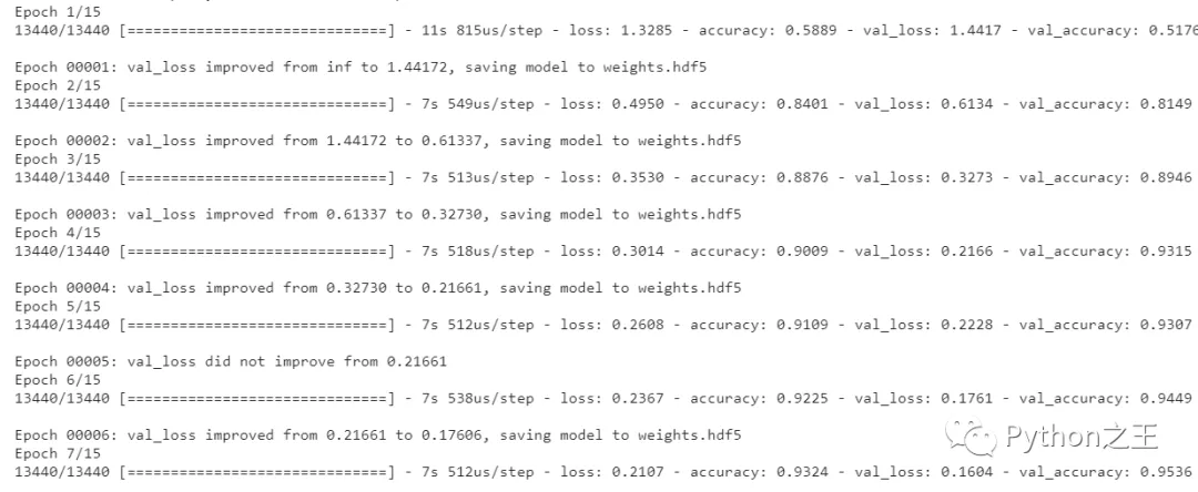
訓練模型，使用batch_size=20來訓練模型，對模型進行15個epochs階段的訓練。

from keras.callbacks import ModelCheckpoint   
 
# 使用檢查點來保存稍后使用的模型權重。 
checkpointer = ModelCheckpoint(filepath='weights.hdf5', verbose=1, save_best_only=True) 
history = model.fit(training_letters_images_scaled, training_letters_labels_encoded,validation_data=(testing_letters_images_scaled,testing_letters_labels_encoded),epochs=15, batch_size=20, verbose=1, callbacks=[checkpointer]) 

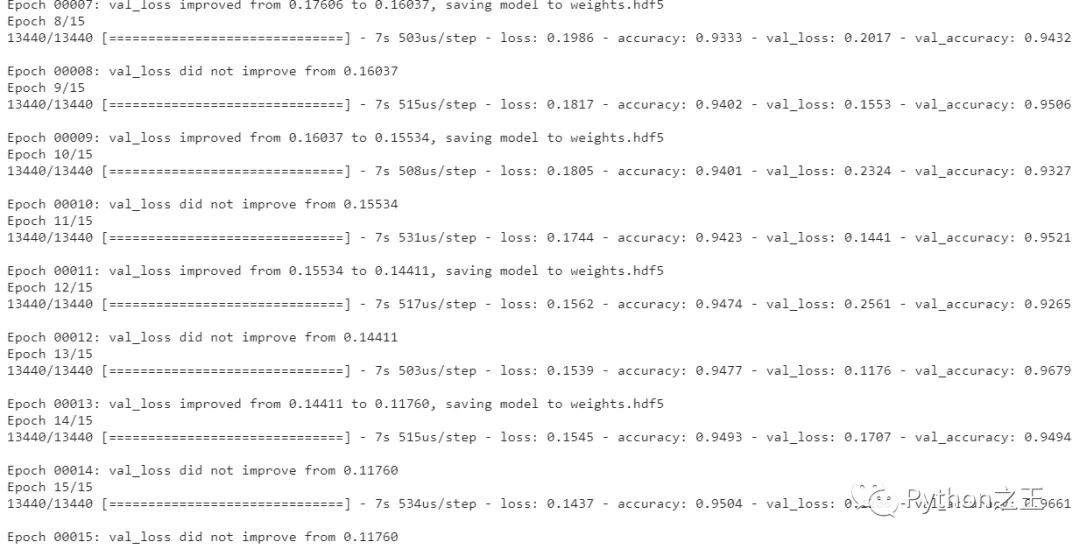
訓練結果如下所示：

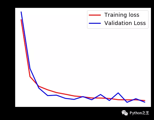
最后Epochs繪制損耗和精度曲線。

import matplotlib.pyplot as plt 
 
def plot_loss_accuracy(history): 
    # Loss  
    plt.figure(figsize=[8,6]) 
    plt.plot(history.history['loss'],'r',linewidth=3.0) 
    plt.plot(history.history['val_loss'],'b',linewidth=3.0) 
    plt.legend(['Training loss', 'Validation Loss'],fontsize=18) 
    plt.xlabel('Epochs ',fontsize=16) 
    plt.ylabel('Loss',fontsize=16) 
    plt.title('Loss Curves',fontsize=16) 
 
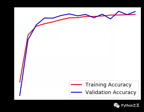
    # Accuracy  
    plt.figure(figsize=[8,6]) 
    plt.plot(history.history['accuracy'],'r',linewidth=3.0) 
    plt.plot(history.history['val_accuracy'],'b',linewidth=3.0) 
    plt.legend(['Training Accuracy', 'Validation Accuracy'],fontsize=18) 
    plt.xlabel('Epochs ',fontsize=16) 
    plt.ylabel('Accuracy',fontsize=16) 
    plt.title('Accuracy Curves',fontsize=16)  
 
plot_loss_accuracy(history) 

「加載具有最佳驗證損失的模型」

# 加載具有最佳驗證損失的模型 
model.load_weights('weights.hdf5') 
metrics = model.evaluate(testing_letters_images_scaled, testing_letters_labels_encoded, verbose=1) 
print("Test Accuracy: {}".format(metrics[1])) 
print("Test Loss: {}".format(metrics[0])) 

輸出如下：

3360/3360 [==============================] - 0s 87us/step 
Test Accuracy: 0.9678571224212646 
Test Loss: 0.11759862171020359 

打印混淆矩陣。

from sklearn.metrics import classification_report 
 
def get_predicted_classes(model, data, labels=None): 
    image_predictions = model.predict(data) 
    predicted_classes = np.argmax(image_predictions, axis=1) 
    true_classes = np.argmax(labels, axis=1) 
    return predicted_classes, true_classes, image_predictions 
 
def get_classification_report(y_true, y_pred): 
    print(classification_report(y_true, y_pred)) 
 
 
y_pred, y_true, image_predictions = get_predicted_classes(model, testing_letters_images_scaled, testing_letters_labels_encoded) 
get_classification_report(y_true, y_pred) 

輸出如下：

          precision    recall  f1-score   support 
 
        0       1.00      0.98      0.99       120 
        1       1.00      0.98      0.99       120 
        2       0.80      0.98      0.88       120 
        3       0.98      0.88      0.93       120 
        4       0.99      0.97      0.98       120 
        5       0.92      0.99      0.96       120 
        6       0.94      0.97      0.95       120 
        7       0.94      0.95      0.95       120 
        8       0.96      0.88      0.92       120 
        9       0.90      1.00      0.94       120 
       10       0.94      0.90      0.92       120 
       11       0.98      1.00      0.99       120 
       12       0.99      0.98      0.99       120 
       13       0.96      0.97      0.97       120 
       14       1.00      0.93      0.97       120 
       15       0.94      0.99      0.97       120 
       16       1.00      0.93      0.96       120 
       17       0.97      0.97      0.97       120 
       18       1.00      0.93      0.96       120 
       19       0.92      0.95      0.93       120 
       20       0.97      0.93      0.94       120 
       21       0.99      0.96      0.97       120 
       22       0.99      0.98      0.99       120 
       23       0.98      0.99      0.99       120 
       24       0.95      0.88      0.91       120 
       25       0.94      0.98      0.96       120 
       26       0.95      0.97      0.96       120 
       27       0.98      0.99      0.99       120 
 
 accuracy                           0.96      3360 
macro avg       0.96      0.96      0.96      3360 
ghted avg       0.96      0.96      0.96      3360 

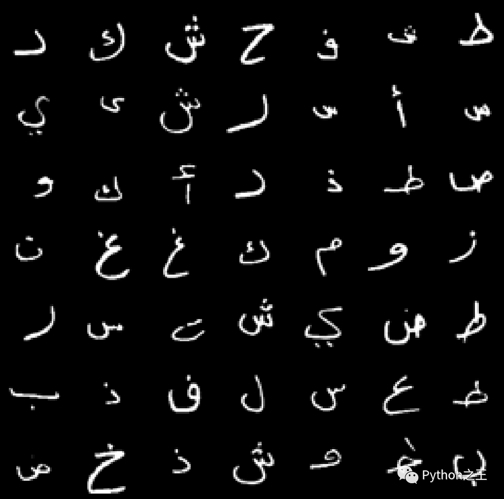
最后繪制隨機幾個相關預測的圖片

indices = np.random.randint(0, testing_letters_labels.shape[0], size=49) 
y_pred = np.argmax(model.predict(training_letters_images_scaled), axis=1) 
 
for i, idx in enumerate(indices): 
    plt.subplot(7,7,i+1) 
         
    image_array = training_letters_images_scaled[idx][:,:,0] 
    image_array = np.flip(image_array, 0) 
    image_array = rotate(image_array, -90) 
        
    plt.imshow(image_array, cmap='gray') 
    plt.title("Pred: {} - Label: {}".format(y_pred[idx], (training_letters_labels[idx] -1))) 
    plt.xticks([]) 
    plt.yticks([]) 
plt.show()