在未來的三年內，深度學習將改變前端開發現狀——它會提高原型設計的速度，并將降低軟件開發的門檻。

繼去年Tony Beltramelli和Airbnb推出了pix2code和ketch2code的論文之后，這個領域就開始騰飛。現在自動化前端開發的最大瓶頸是計算能力，但是通過深度學習算法以及綜合的訓練數據集，我們已然可以開始探索人工前端自動化。

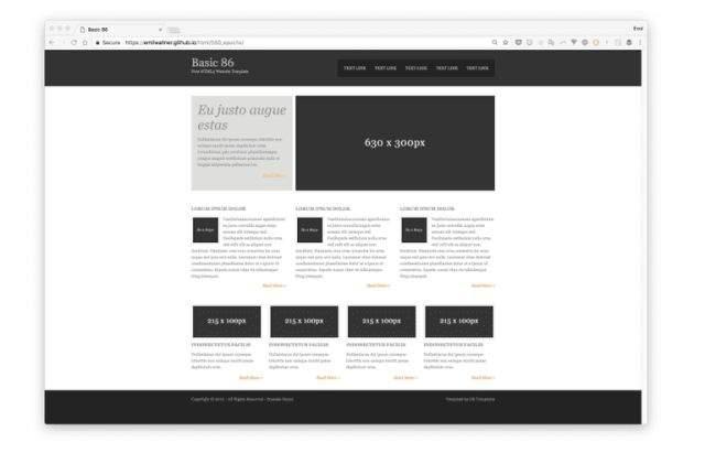
本文我們將通過訓練一個神經網絡，使它可以直接將網頁的設計原型圖轉換成基本的HTML和CSS網頁。

以下是這個訓練過程的簡要概述：

1）將網頁設計圖導入到訓練后的神經網絡中

2）HTML標記

3）展示結果

“我們將構建三個版本的神經網絡”

在第一個版本，我們將實現一個最低限度版本，了解動態這部分的竅門。

HTML版本著重于全過程自動化，并且會解釋各個神經網絡層。最后Bootstrap版中，我們會創建基于LSTM的模型。

這篇文章里的模型都是以Beltramelli的pix2code論文和Brownlee的圖像標注教程。這篇文章的代碼用Python和Keras(基于TensorFlow)完成的。

如果你還是個深度學習領域的新手，那我建議你先了解一下Python,反向傳播算法和卷積神經網絡。我之前的三篇文章可以幫助你開始了解。

核心邏輯

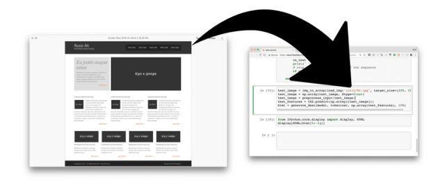
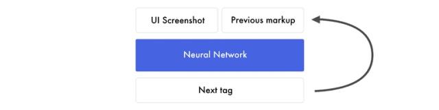
讓我們重新回顧一下我們的目標：我們想要構建一個能夠將網頁截圖轉換成相應HTML/CSS代碼的神經網絡。

我們提供給神經網絡網頁截圖和相對應的HTML代碼來訓練它。.它逐個預測匹配的HTML標簽來學習。當它要預測下一個標簽時，會收到網頁截圖及對應的完整標簽，直到下一個標簽開始。谷歌表格提供了一個簡單的訓練數據的例子創建一個逐詞預測模型是當今最常見的方法。當然還有其他的方法(https://machinelearningmastery.com/deep-learning-caption-generation-models/)，但在整個教程中我們還是會使用的逐詞預測的模型。

請注意，由于對它的每個預測我們都使用同樣的網頁截圖，所以如果我們需要它預測20個詞，那么就需要給它看20遍這個設計原型（即網頁截圖）。現在不要在意神經網絡是如何工作的，我們的重點應該放在神經網絡的輸入輸出參數上。

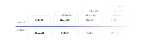
讓我們把重點放在前面的標簽。假設我們訓練神經網絡來預測“I can code"這句話。當它收到"I"時，它會預測到”can" 。接著它會收到"I can“并預測到”code"。它接收之前所有的單詞然后只需要預測下一個單詞。

數據讓神經網絡可以創建特征。特征讓輸入數據和輸出數據有了聯系。神經網絡需要將學習的網頁截圖、HTML語法構建出來，用來預測下一個HTML標簽。

無論什么用途，訓練模型的方式總是相似的。在每一次迭代中使用相同的圖片生成一段段代碼。我們并不會輸入正確的HTML標簽給神經網絡，它使用自已生成的標簽來預測下段標簽。預測在“開始標簽”時初始化，當它預測到“結束標簽”或達到上限時結束。Google Sheet上有另一個示例。

“Hello World!"版本

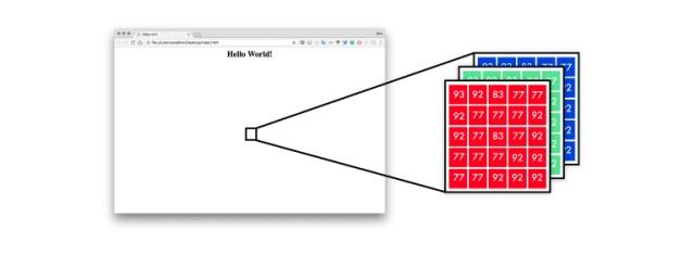
讓我們來構建”Hello World"版本。我們提供給神經網絡一張顯示"Hello World"的網頁截圖并教它如何生成對應的標簽。

首先，神經網絡將設計模型映射成像素值列表。像素值為0-255，其三個通道為紅、黃、藍。

為了使神經網絡能夠理解標簽，我使用獨熱編碼，所以”I can code"會被映射成下圖這個樣子：

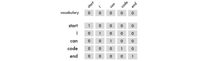
如上圖所示，我們引入了開始標簽和結束標簽，它們能夠幫助神經網絡預測從哪里開始到哪里結束。我們使用順序詞組做為輸入，它是從第一個詞開始，順序連接后面的詞。輸出總是一個詞。

順序詞組的邏輯和詞是一樣的，不過它們需要相同的詞組長度。

它們不受詞匯表的限制，但受到最長詞組長度的限制。如果它比最長詞組長度短，你需要用空詞去補全它，空詞是內容全為0的詞。

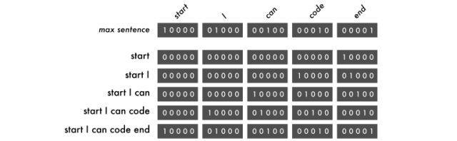
如你所見，空詞是填充在左側的。這樣每次訓練都會改變詞的位置，使得模型能夠學會這句話而不是記住每個單詞的位置。下圖每一行均表示一次預測，共有四次預測。逗號左邊是用RGB表示的圖片，逗號右邊是前面詞，括號外從上到下分別是每個預測的結果，其中結束標簽用紅色方塊表示。

 

#Length of longest sentence max_caption_len = 3 #Size of vocabularyvocab_size = 3 # Load one screenshot for each word and turn them into digits images = for i in range(2): images.append(img_to_array(load_img('screenshot.jpg', target_size=(224,224)))) images = np.array(images, dtype=float) # Preprocess input for the VGG16 model images = preprocess_input(images) #Turn start tokens into one-hot encoding html_input = np.array( [[[0., 0., 0.], #start [0., 0., 0.], [1., 0., 0.]], [[0., 0., 0.], #start Hello World! [1., 0.,0.0., 1., 0.]]]) #Turn next word into one-hot encoding next_words = np.array( [[0., 1., 0.], # Hello World! [0., 0., 1.]]) # end# Load the VGG16 model trained on imagenet and output the classification feature VGG = VGG16(weights='imagenet', include_top=True) # Extract thefeatures from the image features = VGG.predict(images) #Load the feature to the network, apply a dense layer, and repeat the vector vgg_feature = Input(shape=(1000,)) vgg_feature_dense = Dense(5)(vgg_feature) vgg_feature_repeat = RepeatVector(max_caption_len)(vgg_feature_dense) # Extract information from the input seqence language_input = Input(shape=(vocab_size, vocab_size)) language_model = LSTM(5, return_sequences=True)(language_input) # Concatenate the information from the image and the input decoder = concatenate([vgg_feature_repeat, language_model]) # Extract information from the concatenated output decoder = LSTM(5, return_sequences=False)(decoder) # Predict which word comes nextdecoder_output = Dense(vocab_size, activation='softmax')(decoder) # Compile and run the neural network model = Model(inputs=[vgg_feature, language_input], outputs=decoder_output) model.compile(loss='categorical_crossentropy', optimizer='rmsprop') # Train the neural network model.fit([features, html_input], next_words, batch_size=2, shuffle=False, epochs=1000)

在“Hello World"版本中，我們使用三個詞條："start"、"Hello World!"和"end"。

用字符、單詞或者句子作為詞條都是可以的。使用字符作為詞條需要小量的詞匯表，但是會壓垮神經網絡。三者中用單詞作為詞條最佳。

讓我們開始預測吧：

 

# Create an empty sentence and insert the start token sentence = np.zeros((1, 3, 3)) # [[0,0,0], [0,0,0], [0,0,0]] start_token = [1., 0., 0.] # start sentence[0][2] = start_token # place start in empty sentence # Making the first prediction with the start token second_word = model.predict([np.array([features[1]]), sentence]) # Put the second word in the sentence and make the final prediction sentence[0][1] = start_token sentence[0][2] = np.round(second_word) third_word = model.predict([np.array([features[1]]), sentence]) # Place the start token and our two predictions in the sentence sentence[0][0] = start_token sentence[0][1] = np.round(second_word) sentence[0][2] = np.round(third_word) # Transform our one-hot predictions into the final tokens vocabulary = ["start", " 
 
Hello World! 
 
", "end"] for i in sentence[0]: print(vocabulary[np.argmax(i)], end=' ') 

輸出：

 

10 epochs: start start start 
 
100 epochs: start <HTML><center><H1>Hello World!</H1></center></HTML> <HTML><center><H1>Hello World!</H1></center></HTML> 
 
300 epochs: start <HTML><center><H1>Hello World!</H1></center></HTML> end 

 

走過的彎路：

• 在收集數據之前構建第一個運行的版本。在這個項目的早期，我設法得到Geocities托管網站的一個舊版本。它有3800萬個網站。我只顧著這個數據的巨大的可能性，忽視了減少100K大小詞匯所需的巨大工作量。

• 處理一個TB級的數據需要很好的硬件或者很強的耐心。在我的Mac遇到幾個問題后，我最終使用了一個功能強大的遠程服務器。要想獲得順暢的工作流程，估計你得租一個8核CPU的設備，再加上1GPS的網速

• 直到我理解了輸入和輸出數據之后，一切才變得有意義起來。輸入數據X是網頁截圖和之前的標簽。輸出數據Y是下一個標簽。當我明白了這個時，理解它們之間的一切變得更容易了。嘗試不同的體系結構也變得更加容易。

• 別鉆牛角尖。因為這個項目在深度學習中與很多領域相交叉，所以我一路鉆了很多牛角尖。我花了一個星期從頭開始編寫RNN，也對嵌入向量空間感到非常著迷，并且被它獨特的實現方法誘惑了。

• 圖片到編碼的網絡是偽裝了的圖像描述模型。即使當我了解到這一點，我仍然忽視了許多圖像描述的論文，只是因為它們不太酷。但是一旦我了解一些這方面的觀點，我就加快了對問題空間的了解。

在FloygdHub上運行代碼

FloydHub是一個深度學習的培訓平臺。我在剛開始學習深度學習的時候發現了這個平臺，而且用它來訓練和管理我的深度學習實驗。你可以安裝FloydHub，在10分鐘內你就可以運行你的第一個模型了。這是云端GPU運行模型的最佳選擇。

如果你是FloydHub的新手，那么做2分鐘的安裝(https://www.floydhub.com/)或5分鐘的演練(https://www.youtube.com/watch?v=byLQ9kgjTdQ&t=21s)。

克隆存儲庫

git clone https://github.com/emilwallner/Screenshot-to-code-in-Keras.git

登錄并啟動FloydHub命令行工具

cd Screenshot-to-code-in-Keras 
 
floyd login 
 
floyd init s2c: 

在FloydHub云GPU機器上運行一個Jupyter Notebook：

floyd run --gpu --env tensorflow-1.4 --data emilwallner/datasets/imagetocode/2:data --mode jupyter

所有筆記本都在floydhub目錄中。本地東西在本地。運行之后，你可以在這個地址找到第一個筆記本：

floydhub / Hello world / hello world.ipynb。

如果你想要更詳細的說明和標志的解釋，請關注我以前的帖子(https://blog.floydhub.com/colorizing-b&w-photos-with-neural-networks/)。

HTML版本

在這個版本中，我們將自動執行Hello World模型的多個步驟。本部分將著重于創建一個可擴展的實現和神經網絡中的活動部分。

這個版本達不到隨便給一個網站就能推演HTML代碼，但它仍然為我們探索動態問題提供了一個不錯的思路。

概覽

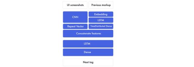
如果我們展開先前圖形的組件，看起來就會像這樣。

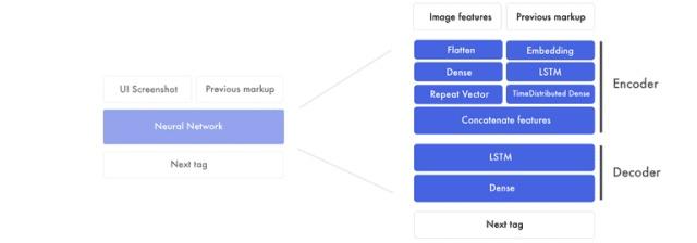
這個版本主要由兩部分組成：

1.首先用于創建圖像特征和之前標簽特征的編碼器。特征是神經網絡創建的用來連接設計原型和標簽的構建塊。在編碼器的結束部分，我們將圖像特征和對應的標簽串起來。

2.然后解碼器將用合并后的設計原型特征和標簽特征來創建下一個標簽特征。這個特征運行在一個全連接神經網絡上。

設計原型特征

由于每一個詞前我們都需要插入一張網頁截圖，它成了訓練神經網絡的瓶頸 (example)(https://docs.google.com/spreadsheets/d/1xXwarcQZAHluorveZsACtXRdmNFbwGtN3WMNhcTdEyQ/edit#gid=0)。所以我們不使用圖像，我們僅提取我們需要的信息來生成標簽。

這是通過一個已經預先在Imagenet上訓練好的卷積神經網絡（CNN）來完成的。在最后的分類前我們需要從神經網絡層中提取特征。

最終的特征是1536個8*8像素的圖片集。雖然我們很難理解這些內容，但是神經網絡可以從這里面提取物體的位置和元素。

HTML標簽特征

在“Hello World”版本中，我們使用獨熱編碼來表示標簽。在這個版本中，我們使用詞嵌入作為輸入，輸出數據仍保持獨熱編碼格式。

句子的數據結構是一樣的，不過映射詞條的方式是不一樣的。獨熱編碼將每個詞都當作獨立部分。相反，我們將輸入的詞轉化成數字列表來表示標簽之間的關系。

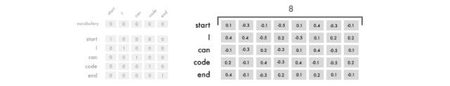
詞嵌入是8維的,根據詞匯量的大小，變化通常在50-500之間。代表詞的8個數字代表權重就像原始神經網絡（vanilla neural network)一樣。它們會不斷地調整以表示詞與詞之間的關系。

這就是我們開始開發標簽特征的方法。在神經網絡中特征被開發出來用來表示輸入數據和輸出數據之間的關系。先不用擔心它們是什么，我們在后面會深入講解。

編碼器

我們會將詞嵌入傳入到LTSM中，它會返回連續的標簽特征。它們通過時序全連接層（time dense layer)運行 -把它想成有多個輸入輸出的全連接層。

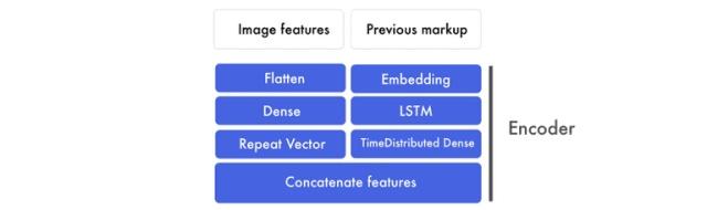
同時圖像特征也被提取出來。無論圖像以哪種數據結構表示，它們都會被展開成一個很長的向量，再傳送到全連接層，提取出高級特征。然后將這些特征與標簽特征級聯起來。

這個過程比較復雜 -讓我們一步步來

標簽特征

這里我們把詞嵌入傳輸到LSTM層。如下圖所示，所有的句子都被填充成長度為3的詞符。

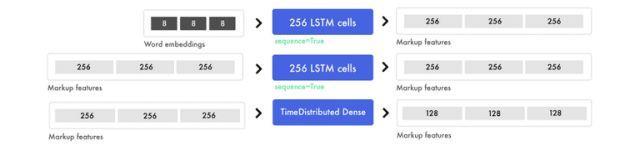
為了混合信號及發現高級模式，我們引入一個TimeDistributed全連接層到標簽特征中。TimeDistributed全連接層和通常的全連接層相似，只不過有很多的輸入和輸出。

圖像特征

同時我們會準備好圖片。我們將這些圖片特征轉換成一個長列表。這些信息并沒有發生變化，只是結構不同罷了。

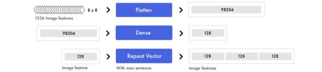
同樣的，為了混合信號并且提取高級概念我們再引入全連接層。由于我們只需要處理一個輸入值，所以一個普通的全連接層就行了。為了連接圖像特征和標簽特征，我們復制圖像特征。

級聯圖像特征和標簽特征

所有的句子都被填充以創建3個標簽特征。由于我們已經準備好了圖像特征，現在我們可以為每個標簽特征添加圖像特征。

在為每個標簽特征添加圖像特征后，我們得到3個圖像-標簽特征。我們會把它們傳輸到解碼器中。

解碼器

這里我們使用剛才得到的圖像-標記結合特征來預測下一個標簽。

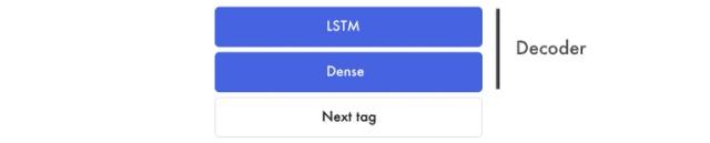
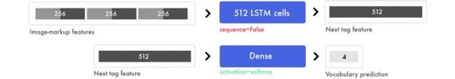
在下面的例子里，我們用這三個圖像-標記特征對來輸出下一個標簽特征。請注意LSTM層將序列設置為“否”，也就是說它僅會預測出一個合并特性，而不是返回同輸入序列同樣長度的特性描述序列。在我們的實際案例中，這就是下一個標簽的特性。它包含了最終預測結果所需要的信息。

最終預測

全連接層所起的作用就相當于一個傳統的前饋型神經網絡。

它將下個標簽特性所包含的512個數位與4個最終預測值聯系起來。假設詞匯表中有四個單詞：start，hello，world以及end。

對于詞匯表中詞匯的預測值可能是[0.1, 0.1, 0.1, 0.7]，在全連接層啟用softmax函數，將概率在0-1的區間內進行離散，同時所有預測值和為1。在本例中，預測第四個單詞即為下一個標簽。之后使用解碼器，將獨熱編碼的結果[0,0,0,1]譯為映射值當中的“end”。

# Load the images and preprocess them for inception-resnet images = all_filenames = listdir('images/') all_filenames.sort for filename inall_filenames: images.append(img_to_array(load_img('images/'+filename, target_size=(299, 299)))) images = np.array(images, dtype=float) images = preprocess_input(images) # Run the images through inception-resnet and extract the features without the classification layer IR2 = InceptionResNetV2(weights='imagenet', include_top=False) features = IR2.predict(images) # We will cap each input sequence to 100 tokensmax_caption_len = 100 # Initialize the function that will create our vocabulary tokenizer = Tokenizer(filters='', split=" ", lower=False) # Read a document and return a string defload_doc(filename): file = open(filename, 'r') text = file.read file.close return text # Load all the HTML files X = all_filenames = listdir('html/'for filename inall_filenames: X.append(load_doc('html/'+filename)) # Create the vocabulary from the html files tokenizer.fit_on_texts(X) # Add +1 to leave space for empty words vocab_size = len(tokenizer.word_index) + 1 # Translate each word in text file to the matching vocabulary indexsequences = tokenizer.texts_to_sequences(X) # The longest HTML filemax_length = max(len(s) for s in sequences) # Intialize our final input to the model X, y, image_data = list, list, list for img_no, seq inenumerate(sequences): for i in range(1, len(seq)): # Add the entire sequence to the input and only keep the next word for the output in_seq, out_seq = seq[:i], seq[i] # If the sentence is shorter than max_length, fill it up with empty words in_seq = pad_sequences([in_seq], maxlen=max_length)[0] # Map the output to one-hot encoding out_seq = to_categorical([out_seq], num_classes=vocab_size)[0] # Add and image corresponding to the HTML file image_data.append(features[img_no]) # Cut the input sentence to 100 tokens, and add it to the input dataX.append(in_seq[-100:]) y.append(out_seq) X, y, image_data = np.array(X), np.array(y), np.array(image_data) # Create the encoder image_features = Input(shape=(8, 8, 1536,)) image_flat = Flatten(image_features) image_flat = Dense(128, activation='relu')(image_flat) ir2_out = RepeatVector(max_caption_len)(image_flat) language_input = Input(shape=(max_caption_len,)) language_model = Embedding(vocab_size, 200, input_length=max_caption_len)(language_input) language_model = LSTM(256, return_sequences=True)(language_model) language_model = LSTM(256, return_sequences=True)(language_model) language_model = TimeDistributed(Dense(128, activation='relu'))(language_model) # Create the decoder decoder = concatenate([ir2_out, language_model]) decoder = LSTM(512, return_sequences=False)(decoder) decoder_output = Dense(vocab_size, activation='softmax')(decoder) # Compile the model model = Model(inputs=[image_features, language_input], outputs=decoder_output) model.compile(loss='categorical_crossentropy', optimizer='rmsprop') # Train the neural network model.fit([image_data, X], y, batch_size=64, shuffle=False, epochs=2) # map an integer to a worddefword_for_id(integer, tokenizer): for word, index intokenizer.word_index.items: if index == integer: return word returnNone # generate a description for an image defgenerate_desc(model, tokenizer, photo, max_length): # seed the generation process in_text = 'START' # iterate over the whole length of the sequence for i in range(900): # integer encode input sequence sequence = tokenizer.texts_to_sequences([in_text])[0][-100:] # pad input sequence = pad_sequences([sequence], maxlen=max_length) # predict next word yhat = model.predict([photo,sequence], verbose=0) # convert probability to integer yhat = np.argmax(yhat) # map integer to word word = word_for_id(yhat, tokenizer) # stop if we cannot map the word if wordisNone: break # append as input for generating the next word in_text += ' ' + word # Print the prediction print(' ' + word, end='') # stop if we predict the end of the sequence if word == 'END': break return # Load and image, preprocess it for IR2, extract features and generate the HTMLtest_image = img_to_array(load_img('images/87.jpg', target_size=(299,299))) test_image = np.array(test_image, dtype=float) test_image = preprocess_input(test_image) test_features = IR2.predict(np.array([test_image])) generate_desc(model, tokenizer, np.array(test_features), 100)

輸出

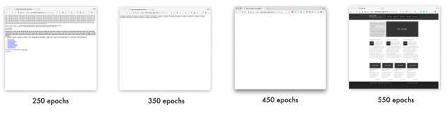
生成的網站鏈接：

• 250 epochs(https://emilwallner.github.io/html/250_epochs/)

• 350 epochs(https://emilwallner.github.io/html/350_epochs/)

• 450 epochs(https://emilwallner.github.io/html/450_epochs/)

• 550 epochs(https://emilwallner.github.io/html/550_epochs/)

如果點擊鏈接無法顯示任何結果，你可以右擊選擇“查看網頁源代碼”。以下是案例中用于識別分析的原網站。

如果上面的鏈接打開后沒有內容顯示，你可以右鍵選擇"查看網頁源代碼“。這里是這些網頁的本來的源代碼。

走過的彎路：

• （對我來說）LSTM網絡的學習困難程度遠高于卷積神經網絡。在我全面認識理解LSTM網絡之后，這一結構對我來說變得容易了一些。Fast.ai的循環神經網絡視頻有極大的幫助。同時在你試圖理解這個網絡結構如何運行的前，也要仔細觀察那些輸入和輸出的特征。

• 從頭構建一個詞庫比起壓縮一個巨大的詞庫要容易太多，因為后者涉及到字體、DIV大小、十六進制顏色編碼、變量名稱和網頁內容。

• 通常文本文件內容是用空格分開的，但是在代碼文件中，你需要自定義解析方法。

• 你可以提取用Imagenet上已經訓練好的模型來提取特征。Imagenet幾乎沒有什么網頁圖片，這可能有違直覺。但是同pix2code的模型比起來，它的損失要高30%。當然我也對基于網頁截圖來預訓練的inception-resnet模型很有興趣。

Bootstrap版本

在我們的最終版本中，我們會使用pix2code論文中搭建的bootstrap網站的一個數據集。通過使用Twitter的bootstrap，可以將HML和CSS相結合，并且壓縮詞庫的大小。

我們將讓它為一副之前沒有見過的網頁截圖生成標簽，同時也會深入探討它是如何建立關于截圖與標記的認知。

我們將會使用17個經過簡化的詞條將這些記號轉換為HTML和CSS，而不是利用bootstrap標簽進行訓練。這一套數據集包括1500個測試截圖以及250幅驗證圖像。平均每個截圖都有65個詞條，結果總計產生96925個訓練樣本。

通過對pix2code論文中提及模型的微調，我們的模型對于網頁組件預測的準確度可以高達97%（基于BLEU飽和搜索測評，詳解見后）。

端到端方法

利用預訓練過的模型提取特征對于圖像標注模型效果的確很好。但經過幾次試驗之后，我發現pix2code的端到端方法對于這類問題效果更佳。預訓練模型并不是通過網頁數據訓練，而是通過定制的分類器訓練。

在這一模型中，我們用一個輕量的卷積神經網絡替換了預訓練得到的圖像特征。我們通過增加步長來增加信息密度，而不是最大池化函數。這樣能最大程度保留前端各元素的位置和顏色信息。

有兩個核心模型可以做到這一點，卷積神經網絡（CNN）和循環神經網絡（RNN）。最常用的循環神經網絡是長短期記憶網絡（LSTM），接下來我將會用到。在我之前的文章中，也總結過許多非常棒的CNN教程，在本案例中，我們重點使用LSTM。

理解LSTM的時間步

掌握LSTM的難點在于時間步。一個原始神經網絡（vanilla neural network)可以看做有兩個時間步。如果你輸入“Hello”，它將預測“World”。但是它嘗試去預測更多的時間步。

在以下的示例中，輸入包含了四個時間步，每一個都對應一個詞。

LSTM適用于含有時間步的輸入，適用于有序信息的神經網絡。如果你對于模型進行解析，它的工作原理看起來類似這樣：每一次向下遞推都保持相同的權重。你可以對于之前的輸出設置一套權重，然后對于新的輸入再設置另一套權重。

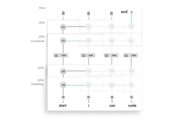
被賦予權重的輸入和輸出將通過激活被聯結并且組合，也就形成了那一時間步的輸出。因為我們會反復使用這些權重，也就會從若干次的輸入中得出信息，并形成對于結果的認知。加權后的輸入和輸出級聯后傳輸給一個激活函數，作為相應的時間步的輸出。這些被復用的權重集描述了輸入的信息，并構建序列的知識。

以下是LSTM模型中每一個時間步的簡化版本。

建議大家參考Andrew Trask的神教程(https://iamtrask.github.io/2015/11/15/anyone-can-code-lstm/)，從無到有搭建一個RNN網絡來理解背后的邏輯

理解LSTM層的單元

每一層LSTM的單元數量決定了它的記憶力，也同樣決定了輸出特征的大小。需要再次指出，我們這里的特征是層與層之間傳遞信息的一長串數字。

LSTM層中的每個單元都保留對于語法不同方面的記錄。下面展示了如何實現一個單元對于div行信息進行保留。這也是我們用于訓練bootstrap模型的一種簡化標記。

每一個LSTM單元都存儲了一個細胞狀態。把細胞狀態看作記憶，權重和激活函數使用不同的方式改變這個狀態。使得LSTM層對于每一次的輸入，可以很好的調整那些信息，決定哪些需要保留，而哪些需要丟棄。

除了傳遞每一次輸入的輸出特征外，層單元也會傳遞細胞狀態，每一個LSTM細胞都對應一個不同的值。如果想了解LSTM層中的要素之間都是如何相互作用的，我強烈推薦Colah的教程，Jayasiri的Numpy實現，Karphay的講座以及評論。

dir_name = 'resources/eval_light/' # Read a file and return a stringdefload_doc(filename): file = open(filename, 'r') text = file.read file.close return text defload_data(data_dir): text = images = # Load all the files and order them all_filenames = listdir(data_dir) all_filenames.sort for filename in (all_filenames): if filename[-3:] =="npz": # Load the images already prepared in arrays image = np.load(data_dir+filename) images.append(image['features']) else: # Load the boostrap tokens and rap them in a start and end tag syntax = ' ' + load_doc(data_dir+filename) + ' ' # Seperate all the words with a single space' '.join(syntax.split) # Add a space after each comma syntax = syntax.replace(',', ' ,') text.append(syntax) images = np.array(images, dtype=float) return images, text train_features, texts = load_data(dir_name) # Initialize the function to create the vocabularytokenizer = Tokenizer(filters='', split=" ", lower=False) # Create the vocabulary tokenizer.fit_on_texts([load_doc('bootstrap.vocab')]) # Add one spot for the empty word in the vocabulary vocab_size = len(tokenizer.word_index) + 1 # Map the input sentences into the vocabulary indexes train_sequences = tokenizer.texts_to_sequences(texts) # The longest set of boostrap tokens max_sequence = max(len(s) for s intrain_sequences) # Specify how many tokens to have in each input sentencemax_length = 48 defpreprocess_data(sequences, features): X, y, image_data = list, list, list for img_no, seq in enumerate(sequences): for i inrange(1, len(seq)): # Add the sentence until the current count(i) and add the current count to the output in_seq, out_seq = seq[:i], seq[i] # Pad all the input token sentences to max_sequence in_seq = pad_sequences([in_seq], maxlen=max_sequence)[0] # Turn the output into one-hot encoding out_seq = to_categorical([out_seq], num_classes=vocab_size)[0] # Add the corresponding image to the boostrap token file image_data.append(features[img_no]) # Cap the input sentence to 48 tokens and add it X.append(in_seq[-48:]) y.append(out_seq) returnnp.array(X), np.array(y), np.array(image_data) X, y, image_data = preprocess_data(train_sequences, train_features) #Create the encoderimage_model = Sequential image_model.add(Conv2D(16, (3, 3), padding='valid', activation='relu', input_shape=(256, 256, 3,))) image_model.add(Conv2D(16, (33), activation='relu', padding='same', strides=2)) image_model.add(Conv2D(32, (33), activation='relu', padding='same'32, (33), activation='relu', padding='same', strides=264, (33), activation='relu', padding='same'64, (33), activation='relu', padding='same', strides=2128, (33), activation='relu', padding='same')) image_model.add(Flatten) image_model.add(Dense(1024, activation='relu')) image_model.add(Dropout(0.3)) image_model.add(Dense(1024, activation='relu'0.3)) image_model.add(RepeatVector(max_length)) visual_input = Input(shape=(256, 256, 3,)) encoded_image = image_model(visual_input) language_input = Input(shape=(max_length,)) language_model = Embedding(vocab_size, 50, input_length=max_length, mask_zero=True)(language_input) language_model = LSTM(128, return_sequences=True)(language_model) language_model = LSTM(128, return_sequences=True)(language_model) #Create the decoder decoder = concatenate([encoded_image, language_model]) decoder = LSTM(512, return_sequences=True)(decoder) decoder = LSTM(512, return_sequences=False)(decoder) decoder = Dense(vocab_size, activation='softmax')(decoder) # Compile the model model = Model(inputs=[visual_input, language_input], outputs=decoder) optimizer = RMSprop(lr=0.0001, clipvalue=1.0) model.compile(loss='categorical_crossentropy', optimizer=optimizer) #Save the model for every 2nd epoch filepath="org-weights-epoch-{epoch:04d}--val_loss-{val_loss:.4f}--loss-{loss:.4f}.hdf5" checkpoint = ModelCheckpoint(filepath, monitor='val_loss', verbose=1, save_weights_only=True, period=2) callbacks_list = [checkpoint] # Train the model model.fit([image_data, X], y, batch_size=64, shuffle=False, validation_split=0.1, callbacks=callbacks_list, verbose=1, epochs=50)

準確率測試

用一種公平合理的方式測試正確率是比較困難的。假設逐詞對照，如果在同步時有一個詞錯位，也許只能收獲0%的正確率。而如果你刪掉一個符合同步預測的詞，準確率也可能高達99%。

我使用了BLEU測評，這一測評在機器翻譯和圖像標注模型上有很好表現。測評將句子打散為四個n-gram，也就是1-4個詞組成的字符串。在以下的預測中，應該是“code”而不是‘cat’。

最終評分需要將每次打散的成績乘以25%：

(4/5) * 0.25 + (2/4) * 0.25 + (1/3) * 0.25 + (0/2) * 0.25 = 0.2 + 0.125 + 0.083 + 0 = 0.408

求和結果再乘以句子長度做取值補償。因為我們以上的例子中長度取值正確，所以這就是我們最終測評分數。

你可以通過增加n-gram的組數來增加測評難度，分為4組n-gram的模型是最符合人類的直覺。建議大家利用以下的代碼運行一些案例，然后讀一讀維基百科對于BLEU測評的描述。

#Create a function to read a file and return its contentdefload_doc(filename): file = open(filename, 'r') text = file.read file.close return text defload_data(data_dir): text = images = files_in_folder = os.listdir(data_dir) files_in_folder.sort for filenamein tqdm(files_in_folder): #Add an image if filename[-3:] == "npz": image = np.load(data_dir+filename) images.append(image['features']) else: # Add text and wrap it in a start and end tag syntax = ' ' + load_doc(data_dir+filename) + ' ' #Seperate each word with a space' '.join(syntax.split) #Add a space between each comma syntax = syntax.replace(',', ' ,') text.append(syntax) images = np.array(images, dtype=float) return images, text #Intialize the function to create the vocabulary tokenizer = Tokenizer(filters='', split=" ", lower=False)#Create the vocabulary in a specific ordertokenizer.fit_on_texts([load_doc('bootstrap.vocab')]) dir_name ='../../../../eval/' train_features, texts = load_data(dir_name) #load model and weights json_file = open('../../../../model.json', 'r') loaded_model_json = json_file.read json_file.close loaded_model = model_from_json(loaded_model_json) # load weights into new modelloaded_model.load_weights("../../../../weights.hdf5") print("Loaded model from disk") # map an integer to a word defword_for_id(integer, tokenizer):for word, index in tokenizer.word_index.items: if index == integer: returnword returnNone print(word_for_id(17, tokenizer)) # generate a description for an image defgenerate_desc(model, tokenizer, photo, max_length): photo = np.array([photo]) # seed the generation process in_text = ' ' # iterate over the whole length of the sequence print(' Prediction---->  ', end='') for i in range(150): # integer encode input sequence sequence = tokenizer.texts_to_sequences([in_text])[0] # pad inputsequence = pad_sequences([sequence], maxlen=max_length) # predict next word yhat = loaded_model.predict([photo, sequence], verbose=0) # convert probability to integer yhat = argmax(yhat) # map integer to word word = word_for_id(yhat, tokenizer) # stop if we cannot map the word if wordisNone: break # append as input for generating the next word in_text += word + ' ' # stop if we predict the end of the sequence print(word + ' ', end='') if word == '': break return in_text max_length = 48 # evaluate the skill of the model defevaluate_model(model, descriptions, photos, tokenizer, max_length): actual, predicted = list, list # step over the whole set for i in range(len(texts)): yhat = generate_desc(model, tokenizer, photos[i], max_length) # store actual and predictedprint(' Real----> ' + texts[i]) actual.append([texts[i].split]) predicted.append(yhat.split) # calculate BLEU score bleu = corpus_bleu(actual, predicted) return bleu, actual, predicted bleu, actual, predicted = evaluate_model(loaded_model, texts, train_features, tokenizer, max_length) #Compile the tokens into HTML and css dsl_path ="compiler/assets/web-dsl-mapping.json" compiler = Compiler(dsl_path) compiled_website = compiler.compile(predicted[0], 'index.html') print(compiled_website ) print(bleu)

輸出

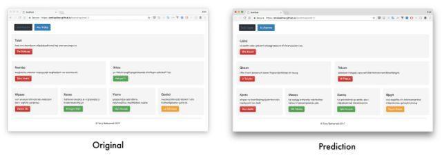
輸出樣本鏈接：

• Generated website 1 - Original 1

  (https://emilwallner.github.io/bootstrap/pred_1/) (https://emilwallner.github.io/bootstrap/real_1/)

• Generated website 2 - Original 2

  () ()

• Generated website 3 - Original 3

  () ()

• Generated website 4 - Original 4

  () ()

• Generated website 5 - Original 5

  () ()

走過的彎路：

• 理解每個模型的不足，而不是隨機選擇模型測試。一開始我采用的方法比較隨機，比如批量歸一化,雙向網絡，甚至嘗試實現注意力。看到測試數據后，我才明白這些方法并不能準確的預測顏色和位置，這是我意識到卷積神經網絡當中存在一些不足。這導致我使用增加步長的辦法去代替最大池化方法。損失從0.12降到了0.02，同時BLEU評分從85%升到97%。

• 如果具有相關性的話，僅考慮使用經過預訓練的模型。對于小型的數據集，我認為一個經過訓練的圖像模型可以改善表現。以我個人的經驗看來，一個端到端的模型訓練費時，并且需要更多的內存，但是準確率會提高30%。

• 如果使用遠程服務器運行模型，需要考慮到輕微的偏差。我的MAC以字母表順序讀取文件，但是在服務器上，文件是隨機讀取的。這會導致截圖和代碼之間的不匹配。雖然預測結果趨同，但是有效數據比起重新匹配前要糟糕50%。

• 掌握引用的庫函數。包括詞匯表中的空詞條里的填充空格。如果不進行特別添加，識別中將不包括這一標記。我是通過幾次觀察到最終結果中無法預測出“單個”標記，才注意到這一點。快速檢查一遍后，我意識到這并不包含在詞庫中。同時也需要注意，訓練和檢測時，需要使用同樣順序的詞庫。

• 實驗時使用輕量的模型。利用GRU而不是LSTM可以讓每光華迭代循環的時間減少30%，并且對于結果不會有太大影響。

[[218148]]

接下會發生什么？

[[218149]]

• 前端開發是應用深度學習理想的空間。生成數據容易，并且現在的深度學習算法可以實現絕大部分的邏輯。

• 其中很有意思的地方是“通過LSTM實現注意力”。它不僅可以用來提高準確率，而且讓我們可以讓CNN將它的注意力放在生成標簽上。

• 注意力也是標簽、樣式、腳本甚至后端之間交流的關鍵。注意力層可以追蹤變量，使神經網格可以在不同的編程語言中交流。

• 但是在不久的將來，最大的影響來自于建立生成數據的可擴展方法。那時你可以一步步地添加字體、顏色、內容和動畫。

• 目前大部分的進步在是將草圖轉換成模板。在兩年內，我們可以在紙上畫上應用的模板，然后瞬間生成對應的前端代碼。事實上Airbnb’s design team(https://airbnb.design/sketching-interfaces/) andUizard(https://www.uizard.io/)已經建立了基本可以使用的原型了。

進一步的實驗

• 根據相應的語法創建一個穩定的隨機應用/網站生成器。

• 生成從草圖到應用的數據。自動轉換應用/網頁截圖到草圖并用GAN來構建多樣性。

• 添加注意力層，可視化每一次預測的焦點，像這個模型一樣。

• 為模塊化方法創建一個框架。比如字體編碼器、顏色編碼器、結構編碼器，然后用一個解碼器將它們整合起來。從穩定的圖像特征開始似乎不錯。

• 讓神經網絡學習簡單的HTML組件，然后將它生成CSS動畫。注意力機制和可視化輸入源真的很神奇。

關于作者： Emil Wallner

深度學習鄰域的資深博客撰寫者，投資人，曾就職于牛津大學商學院，現長期居住在法國，是非盈利組織42(écoles)項目組成員。我們已獲得授權翻譯