機器通過損失函數進行學習。這是一種評估特定算法對給定數據建模程度的方法。如果預測值與實際結果偏離較遠，損失函數會得到一個非常大的值。在一些優化函數的輔助下，損失函數逐漸學會減少預測值的誤差。本文將介紹幾種損失函數及其在機器學習和深度學習領域的應用。

[[243642]]

損失函數和優化

沒有一個適合所有機器學習算法的損失函數。針對特定問題選擇損失函數涉及到許多因素，比如所選機器學習算法的類型、是否易于計算導數以及數據集中異常值所占比例。

從學習任務的類型出發，可以從廣義上將損失函數分為兩大類——回歸損失和分類損失。在分類任務中，我們要從類別值有限的數據集中預測輸出，比如給定一個手寫數字圖像的大數據集，將其分為 0～9 中的一個。而回歸問題處理的則是連續值的預測問題，例如給定房屋面積、房間數量以及房間大小，預測房屋價格。

NOTE  
        n        - Number of training examples. 
        i        - ith training example in a data set. 
        y(i)     - Ground truth label for ith training example. 
        y_hat(i) - Prediction for ith training example. 

回歸損失

1. 均方誤差/平方損失/L2 損失

數學公式：

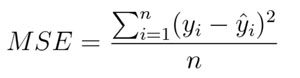
均方誤差

顧名思義，均方誤差(MSE)度量的是預測值和實際觀測值間差的平方的均值。它只考慮誤差的平均大小，不考慮其方向。但由于經過平方，與真實值偏離較多的預測值會比偏離較少的預測值受到更為嚴重的懲罰。再加上 MSE 的數學特性很好，這使得計算梯度變得更容易。

import numpy as np 
y_hat = np.array([0.000, 0.166, 0.333]) 
y_true = np.array([0.000, 0.254, 0.998]) 
def rmse(predictions, targets): 
    differences = predictions - targets 
    differencesdifferences_squared = differences ** 2 
    mean_of_differences_squared = differences_squared.mean() 
    rmse_val = np.sqrt(mean_of_differences_squared) 
    return rmse_val 
print("d is: " + str(["%.8f" % elem for elem in y_hat])) 
print("p is: " + str(["%.8f" % elem for elem in y_true])) 
rmsermse_val = rmse(y_hat, y_true) 
print("rms error is: " + str(rmse_val)) 

2. 平均絕對誤差/L1 損失

數學公式：

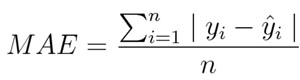
平均絕對誤差

平均絕對誤差(MAE)度量的是預測值和實際觀測值之間絕對差之和的平均值。和 MSE 一樣，這種度量方法也是在不考慮方向的情況下衡量誤差大小。但和 MSE 的不同之處在于，MAE 需要像線性規劃這樣更復雜的工具來計算梯度。此外，MAE 對異常值更加穩健，因為它不使用平方。

import numpy as np 
y_hat = np.array([0.000, 0.166, 0.333]) 
y_true = np.array([0.000, 0.254, 0.998]) 
 
print("d is: " + str(["%.8f" % elem for elem in y_hat])) 
print("p is: " + str(["%.8f" % elem for elem in y_true])) 
 
def mae(predictions, targets): 
    differences = predictions - targets 
    absolute_differences = np.absolute(differences) 
    mean_absolute_differences = absolute_differences.mean() 
    return mean_absolute_differences 
maemae_val = mae(y_hat, y_true) 
print ("mae error is: " + str(mae_val)) 

3. 平均偏差誤差(mean bias error)

與其它損失函數相比，這個函數在機器學習領域沒有那么常見。它與 MAE 相似，唯一的區別是這個函數沒有用絕對值。用這個函數需要注意的一點是，正負誤差可以互相抵消。盡管在實際應用中沒那么準確，但它可以確定模型存在正偏差還是負偏差。

數學公式：

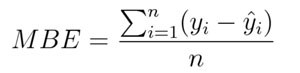
平均偏差誤差

二、分類損失

1. Hinge Loss/多分類 SVM 損失

簡言之，在一定的安全間隔內(通常是 1)，正確類別的分數應高于所有錯誤類別的分數之和。因此 hinge loss 常用于***間隔分類(maximum-margin classification)，最常用的是支持向量機。盡管不可微，但它是一個凸函數，因此可以輕而易舉地使用機器學習領域中常用的凸優化器。

數學公式：

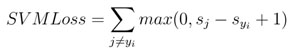
SVM 損失(Hinge Loss)

思考下例，我們有三個訓練樣本，要預測三個類別(狗、貓和馬)。以下是我們通過算法預測出來的每一類的值：

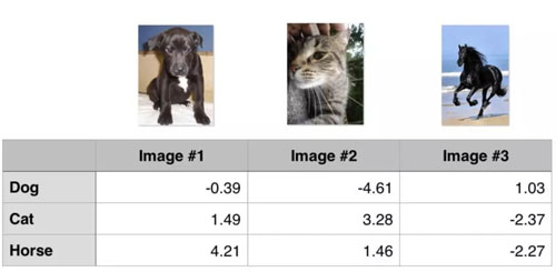
Hinge loss/多分類 SVM 損失

計算這 3 個訓練樣本的 hinge loss：

## 1st training example 
max(0, (1.49) - (-0.39) + 1) + max(0, (4.21) - (-0.39) + 1) 
max(0, 2.88) + max(0, 5.6) 
2.88 + 5.6 
8.48 (High loss as very wrong prediction) 
## 2nd training example 
max(0, (-4.61) - (3.28)+ 1) + max(0, (1.46) - (3.28)+ 1) 
max(0, -6.89) + max(0, -0.82) 
0 + 0 
0 (Zero loss as correct prediction) 
## 3rd training example 
max(0, (1.03) - (-2.27)+ 1) + max(0, (-2.37) - (-2.27)+ 1) 
max(0, 4.3) + max(0, 0.9) 
4.3 + 0.9 
5.2 (High loss as very wrong prediction) 

交叉熵損失/負對數似然：

這是分類問題中最常見的設置。隨著預測概率偏離實際標簽，交叉熵損失會逐漸增加。

數學公式：

交叉熵損失

注意，當實際標簽為 1(y(i)=1) 時，函數的后半部分消失，而當實際標簽是為 0(y(i=0)) 時，函數的前半部分消失。簡言之，我們只是把對真實值類別的實際預測概率的對數相乘。還有重要的一點是，交叉熵損失會重重懲罰那些置信度高但是錯誤的預測值。

import numpy as np 
predictions = np.array([[0.25,0.25,0.25,0.25], 
                        [0.01,0.01,0.01,0.96]]) 
targets = np.array([[0,0,0,1], 
                   [0,0,0,1]]) 
def cross_entropy(predictions, targets, epsilon=1e-10): 
    predictions = np.clip(predictions, epsilon, 1. - epsilon) 
    N = predictions.shape[0] 
    ce_loss = -np.sum(np.sum(targets * np.log(predictions + 1e-5)))/N 
    return ce_loss 
cross_entropycross_entropy_loss = cross_entropy(predictions, targets) 
print ("Cross entropy loss is: " + str(cross_entropy_loss)) 

【本文是51CTO專欄機構“機器之心”的原創文章，微信公眾號“機器之心( id: almosthuman2014)”】

戳這里，看該作者更多好文