如何在表格數據上使用特征提取進行機器學習
數據準備最常見的方法是研究一個數據集,審查機器學習算法的期望,然后仔細選擇最合適的數據準備技術來轉換原始數據,以最好地滿足算法的期望。這是緩慢的,昂貴的,并且需要大量的專業知識。
數據準備的另一種方法是并行地對原始數據應用一套通用和常用的數據準備技術,并將所有轉換的結果合并到一個大數據集中,從中可以擬合和評估模型。
這是數據準備的另一種哲學,它將數據轉換視為一種從原始數據中提取顯著特征的方法,從而將問題的結構暴露給學習算法。它需要學習加權輸入特征可伸縮的算法,并使用那些與被預測目標最相關的輸入特征。
這種方法需要較少的專業知識,與數據準備方法的全網格搜索相比,在計算上是有效的,并且可以幫助發現非直觀的數據準備解決方案,為給定的預測建模問題取得良好或最好的性能。
在本文中,我們將介紹如何使用特征提取對表格數據進行數據準備。
特征提取為表格數據的數據準備提供了另一種方法,其中所有數據轉換都并行應用于原始輸入數據,并組合在一起以創建一個大型數據集。
如何使用特征提取方法進行數據準備,以提高標準分類數據集的基準性能。。
如何將特征選擇添加到特征提取建模管道中,以進一步提升標準數據集上的建模性能。
本文分為三個部分:
一、特征提取技術的數據準備
二、數據集和性能基準
- 葡萄酒分類數據集
- 基準模型性能
三、特征提取方法進行數據準備
特征提取技術的數據準備
數據準備可能具有挑戰性。
最常用和遵循的方法是分析數據集,檢查算法的要求,并轉換原始數據以最好地滿足算法的期望。
這可能是有效的,但也很慢,并且可能需要數據分析和機器學習算法方面的專業知識。
另一種方法是將輸入變量的準備視為建模管道的超參數,并在選擇算法和算法配置時對其進行調優。
盡管它在計算上可能會很昂貴,但它也可能是暴露不直觀的解決方案并且只需要很少的專業知識的有效方法。
在這兩種數據準備方法之間尋求合適的方法是將輸入數據的轉換視為特征工程或特征提取過程。這涉及對原始數據應用一套通用或常用的數據準備技術,然后將所有特征聚合在一起以創建一個大型數據集,然后根據該數據擬合并評估模型。
該方法的原理將每種數據準備技術都視為一種轉換,可以從原始數據中提取顯著特征,以呈現給學習算法。理想情況下,此類轉換可解開復雜的關系和復合輸入變量,進而允許使用更簡單的建模算法,例如線性機器學習技術。
由于缺乏更好的名稱,我們將其稱為“ 特征工程方法 ”或“ 特征提取方法 ”,用于為預測建模項目配置數據準備。
它允許在選擇數據準備方法時使用數據分析和算法專業知識,并可以找到不直觀的解決方案,但計算成本卻低得多。
輸入特征數量的排除也可以通過使用特征選擇技術來明確解決,這些特征選擇技術嘗試對所提取的大量特征的重要性或價值進行排序,并僅選擇與預測目標最相關的一小部分變量。
我們可以通過一個可行的示例探索這種數據準備方法。
在深入研究示例之前,讓我們首先選擇一個標準數據集并制定性能基準。
數據集和性能基準
我們將首先選擇一個標準的機器學習數據集,并為此數據集建立性能基準。這將為探索數據準備的特征提取方法提供背景。
葡萄酒分類數據集
我們將使用葡萄酒分類數據集。
該數據集具有13個輸入變量,這些變量描述了葡萄酒樣品的化學成分,并要求將葡萄酒分類為三種類型之一。
該示例加載數據集并將其拆分為輸入和輸出列,然后匯總數據數組。
- # example of loading and summarizing the wine dataset
- from pandas import read_csv
- # define the location of the dataset
- url = 'https://raw.githubusercontent.com/jbrownlee/Datasets/master/wine.csv'
- # load the dataset as a data frame
- df = read_csv(url, header=None)
- # retrieve the numpy array
- data = df.values
- # split the columns into input and output variables
- X, y = data[:, :-1], data[:, -1]
- # summarize the shape of the loaded data
- print(X.shape, y.shape)
- #(178, 13) (178,)
通過運行示例,我們可以看到數據集已正確加載,并且有179行數據,其中包含13個輸入變量和一個目標變量。
接下來,讓我們在該數據集上評估一個模型,并建立性能基準。
基準模型性能
通過評估原始輸入數據的模型,我們可以為葡萄酒分類任務建立性能基準。
在這種情況下,我們將評估邏輯回歸模型。
首先,如scikit-learn庫所期望的,我們可以通過確保輸入變量是數字并且目標變量是標簽編碼來執行最少的數據準備。
- # minimally prepare dataset
- X = X.astype('float')
- y = LabelEncoder().fit_transform(y.astype('str'))
接下來,我們可以定義我們的預測模型。
- # define the model
- model = LogisticRegression(solver='liblinear')
我們將使用重復分層k-fold交叉驗證的標準(10次重復和3次重復)來評估模型。
模型性能將用分類精度來評估。
- model = LogisticRegression(solver='liblinear')
- # define the cross-validation procedure
- cv = RepeatedStratifiedKFold(n_splits=10, n_repeats=3, random_state=1)
- # evaluate model
- scores = cross_val_score(model, X, y, scoring='accuracy', cv=cv, n_jobs=-1)
在運行結束時,我們將報告所有重復和評估倍數中收集的準確性得分的平均值和標準偏差。
- # report performance
- print('Accuracy: %.3f (%.3f)' % (mean(scores), std(scores)))
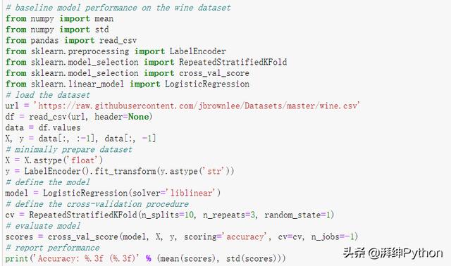
結合在一起,下面列出了在原酒分類數據集上評估邏輯回歸模型的完整示例。
- # baseline model performance on the wine dataset
- from numpy import mean
- from numpy import std
- from pandas import read_csv
- from sklearn.preprocessing import LabelEncoder
- from sklearn.model_selection import RepeatedStratifiedKFold
- from sklearn.model_selection import cross_val_score
- from sklearn.linear_model import LogisticRegression
- # load the dataset
- url = 'https://raw.githubusercontent.com/jbrownlee/Datasets/master/wine.csv'
- df = read_csv(url, header=None)
- data = df.values
- X, y = data[:, :-1], data[:, -1]
- # minimally prepare dataset
- X = X.astype('float')
- y = LabelEncoder().fit_transform(y.astype('str'))
- # define the model
- model = LogisticRegression(solver='liblinear')
- # define the cross-validation procedure
- cv = RepeatedStratifiedKFold(n_splits=10, n_repeats=3, random_state=1)
- # evaluate model
- scores = cross_val_score(model, X, y, scoring='accuracy', cv=cv, n_jobs=-1)
- # report performance
- print('Accuracy: %.3f (%.3f)' % (mean(scores), std(scores)))
- #Accuracy: 0.953 (0.048)
通過運行示例評估模型性能,并報告均值和標準差分類準確性。
考慮到學習算法的隨機性,評估程序以及機器之間的精度差異,您的結果可能會有所不同。嘗試運行該示例幾次。
在這種情況下,我們可以看到,對原始輸入數據進行的邏輯回歸模型擬合獲得了約95.3%的平均分類精度,為性能提供了基準。
接下來,讓我們探討使用基于特征提取的數據準備方法是否可以提高性能。
特征提取方法進行數據準備
第一步是選擇一套通用且常用的數據準備技術。
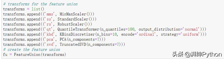
在這種情況下,假設輸入變量是數字,我們將使用一系列轉換來更改輸入變量的比例,例如MinMaxScaler,StandardScaler和RobustScaler,以及使用轉換來鏈接輸入變量的分布,例如QuantileTransformer和KBinsDiscretizer。最后,我們還將使用轉換來消除輸入變量(例如PCA和TruncatedSVD)之間的線性相關性。
FeatureUnion類可用于定義要執行的轉換列表,這些轉換的結果將被聚合在一起。這將創建一個具有大量列的新數據集。
列數的估計將是13個輸入變量乘以五次轉換或65次再加上PCA和SVD維數降低方法的14列輸出,從而得出總共約79個特征。
- # transforms for the feature union
- transforms = list()
- transforms.append(('mms', MinMaxScaler()))
- transforms.append(('ss', StandardScaler()))
- transforms.append(('rs', RobustScaler()))
- transforms.append(('qt', QuantileTransformer(n_quantiles=100, output_distribution='normal')))
- transforms.append(('kbd', KBinsDiscretizer(n_bins=10, encode='ordinal', strategy='uniform')))
- transforms.append(('pca', PCA(n_components=7)))
- transforms.append(('svd', TruncatedSVD(n_components=7)))
- # create the feature union
- fu = FeatureUnion(transforms)
然后,我們可以使用FeatureUnion作為第一步,并使用Logistic回歸模型作為最后一步來創建建模管道。
- # define the model
- model = LogisticRegression(solver='liblinear')
- # define the pipeline
- steps = list()
- steps.append(('fu', fu))
- steps.append(('m', model))
- pipeline = Pipeline(steps=steps)
然后可以像前面一樣使用重復的分層k-fold交叉驗證來評估管道。
下面列出了完整的示例。
- # data preparation as feature engineering for wine dataset
- from numpy import mean
- from numpy import std
- from pandas import read_csv
- from sklearn.model_selection import RepeatedStratifiedKFold
- from sklearn.model_selection import cross_val_score
- from sklearn.linear_model import LogisticRegression
- from sklearn.pipeline import Pipeline
- from sklearn.pipeline import FeatureUnion
- from sklearn.preprocessing import LabelEncoder
- from sklearn.preprocessing import MinMaxScaler
- from sklearn.preprocessing import StandardScaler
- from sklearn.preprocessing import RobustScaler
- from sklearn.preprocessing import QuantileTransformer
- from sklearn.preprocessing import KBinsDiscretizer
- from sklearn.decomposition import PCA
- from sklearn.decomposition import TruncatedSVD
- # load the dataset
- url = 'https://raw.githubusercontent.com/jbrownlee/Datasets/master/wine.csv'
- df = read_csv(url, header=None)
- data = df.values
- X, y = data[:, :-1], data[:, -1]
- # minimally prepare dataset
- X = X.astype('float')
- y = LabelEncoder().fit_transform(y.astype('str'))
- # transforms for the feature union
- transforms = list()
- transforms.append(('mms', MinMaxScaler()))
- transforms.append(('ss', StandardScaler()))
- transforms.append(('rs', RobustScaler()))
- transforms.append(('qt', QuantileTransformer(n_quantiles=100, output_distribution='normal')))
- transforms.append(('kbd', KBinsDiscretizer(n_bins=10, encode='ordinal', strategy='uniform')))
- transforms.append(('pca', PCA(n_components=7)))
- transforms.append(('svd', TruncatedSVD(n_components=7)))
- # create the feature union
- fu = FeatureUnion(transforms)
- # define the model
- model = LogisticRegression(solver='liblinear')
- # define the pipeline
- steps = list()
- steps.append(('fu', fu))
- steps.append(('m', model))
- pipeline = Pipeline(steps=steps)
- # define the cross-validation procedure
- cv = RepeatedStratifiedKFold(n_splits=10, n_repeats=3, random_state=1)
- # evaluate model
- scores = cross_val_score(pipeline, X, y, scoring='accuracy', cv=cv, n_jobs=-1)
- # report performance
- print('Accuracy: %.3f (%.3f)' % (mean(scores), std(scores)))
- #Accuracy: 0.968 (0.037)
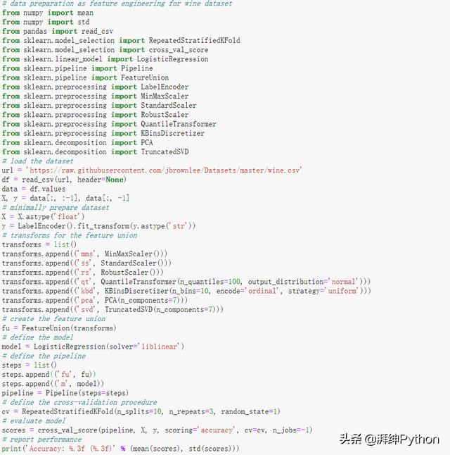
通過運行示例評估模型性能,并報告均值和標準差分類準確性。
考慮到學習算法的隨機性,評估程序以及機器之間的精度差異,您的結果可能會有所不同。嘗試運行該示例幾次。
在這種情況下,我們可以看到性能相對于基準性能有所提升,實現了平均分類精度約96.8%。
嘗試向FeatureUnion添加更多數據準備方法,以查看是否可以提高性能。
我們還可以使用特征選擇將大約80個提取的特征縮減為與模型最相關的特征的子集。除了減少模型的復雜性之外,它還可以通過刪除不相關和冗余的輸入特征來提高性能。
在這種情況下,我們將使用遞歸特征消除(RFE)技術進行特征選擇,并將其配置為選擇15個最相關的特征。
- # define the feature selection
- rfe = RFE(estimator=LogisticRegression(solver='liblinear'), n_features_to_select=15)
然后我們可以將RFE特征選擇添加到FeatureUnion算法之后和LogisticRegression算法之前的建模管道中。
- # define the pipeline
- steps = list()
- steps.append(('fu', fu))
- steps.append(('rfe', rfe))
- steps.append(('m', model))
- pipeline = Pipeline(steps=steps)
將這些結合起來,下面列出了特征選擇的特征選擇數據準備方法的完整示例。
- # data preparation as feature engineering with feature selection for wine dataset
- from numpy import mean
- from numpy import std
- from pandas import read_csv
- from sklearn.model_selection import RepeatedStratifiedKFold
- from sklearn.model_selection import cross_val_score
- from sklearn.linear_model import LogisticRegression
- from sklearn.pipeline import Pipeline
- from sklearn.pipeline import FeatureUnion
- from sklearn.preprocessing import LabelEncoder
- from sklearn.preprocessing import MinMaxScaler
- from sklearn.preprocessing import StandardScaler
- from sklearn.preprocessing import RobustScaler
- from sklearn.preprocessing import QuantileTransformer
- from sklearn.preprocessing import KBinsDiscretizer
- from sklearn.feature_selection import RFE
- from sklearn.decomposition import PCA
- from sklearn.decomposition import TruncatedSVD
- # load the dataset
- url = 'https://raw.githubusercontent.com/jbrownlee/Datasets/master/wine.csv'
- df = read_csv(url, header=None)
- data = df.values
- X, y = data[:, :-1], data[:, -1]
- # minimally prepare dataset
- X = X.astype('float')
- y = LabelEncoder().fit_transform(y.astype('str'))
- # transforms for the feature union
- transforms = list()
- transforms.append(('mms', MinMaxScaler()))
- transforms.append(('ss', StandardScaler()))
- transforms.append(('rs', RobustScaler()))
- transforms.append(('qt', QuantileTransformer(n_quantiles=100, output_distribution='normal')))
- transforms.append(('kbd', KBinsDiscretizer(n_bins=10, encode='ordinal', strategy='uniform')))
- transforms.append(('pca', PCA(n_components=7)))
- transforms.append(('svd', TruncatedSVD(n_components=7)))
- # create the feature union
- fu = FeatureUnion(transforms)
- # define the feature selection
- rfe = RFE(estimator=LogisticRegression(solver='liblinear'), n_features_to_select=15)
- # define the model
- model = LogisticRegression(solver='liblinear')
- # define the pipeline
- steps = list()
- steps.append(('fu', fu))
- steps.append(('rfe', rfe))
- steps.append(('m', model))
- pipeline = Pipeline(steps=steps)
- # define the cross-validation procedure
- cv = RepeatedStratifiedKFold(n_splits=10, n_repeats=3, random_state=1)
- # evaluate model
- scores = cross_val_score(pipeline, X, y, scoring='accuracy', cv=cv, n_jobs=-1)
- # report performance
- print('Accuracy: %.3f (%.3f)' % (mean(scores), std(scores)))
- #Accuracy: 0.989 (0.022)
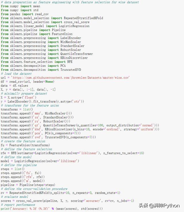
運行實例評估模型的性能,并報告均值和標準差分類精度。
由于學習算法的隨機性、評估過程以及不同機器之間的精度差異,您的結果可能會有所不同。試著運行這個例子幾次。
再一次,我們可以看到性能的進一步提升,從所有提取特征的96.8%提高到建模前使用特征選擇的98.9。