初學者指南:使用Numpy、Keras和PyTorch實現簡單的線性回歸
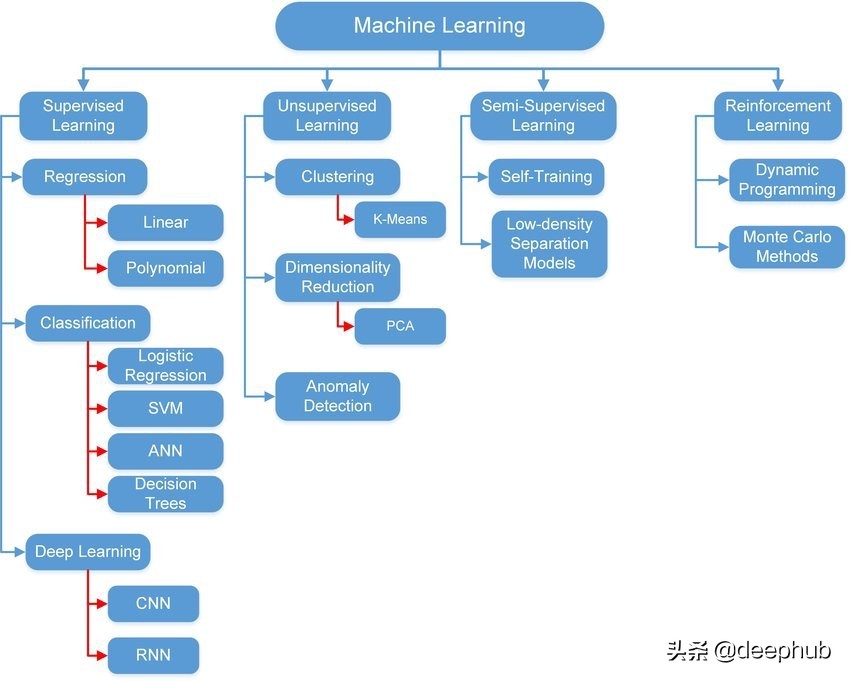
不同類型的機器學習技術可以劃分到不同類別,如圖 1 所示。方法的選擇取決于問題的類型(分類、回歸、聚類)、數據的類型(圖像、圖形、時間系列、音頻等等)以及方法本身的配置(調優)。
在本文中,我們將使用 Python 中最著名的三個模塊來實現一個簡單的線性回歸模型。 使用 Python 的原因是它易于學習和應用。 我們將使用的三個模塊是:
1- Numpy:可以用于數組、矩陣、多維矩陣以及與它們相關的所有操作。
2- Keras:TensorFlow 的高級接口。 它也用于支持和實現深度學習模型和淺層模型。 它是由谷歌工程師開發的。
3- PyTorch:基于 Torch 的深度學習框架。 它是由 Facebook 開發的。
所有這些模塊都是開源的。 Keras 和 PyTorch 都支持使用 GPU 來加快執行速度。
以下部分介紹線性回歸的理論和概念。 如果您已經熟悉理論并且想要實踐部分,可以跳過到下一部分。
線性回歸
它是一種數學方法,可以將一條線與基礎數據擬合。 它假設輸出和輸入之間存在線性關系。 輸入稱為特征或解釋變量,輸出稱為目標或因變量。 輸出變量必須是連續的。 例如,價格、速度、距離和溫度。 以下等式在數學上表示線性回歸模型:
Y = W*X + B
如果把這個方程寫成矩陣形式。 Y 是輸出矩陣,X 是輸入矩陣,W 是權重矩陣,B 是偏置向量。 權重和偏置是線性回歸參數。 有時權重和偏置分別稱為斜率和截距。
訓練該模型的第一步是隨機初始化這些參數。 然后它使用輸入的數據來計算輸出。 通過測量誤差將計算出的輸出與實際輸出進行比較,并相應地更新參數。并重復上述步驟。該誤差稱為 L2 范數(誤差平方和),由下式給出:
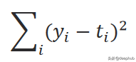
計算誤差的函數又被稱作損失函數,它可以有不同的公式。 i 是數據樣本數,y 是預測輸出,t 是真實目標。 根據以下等式中給出的梯度下降規則更新參數:
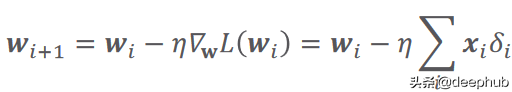
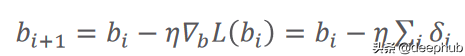
在這里,(希臘字母 eta)是學習率,它指定參數的更新步驟(更新速度)。 (希臘字母 delta)只是預測輸出和真實輸出之間的差異。 i 代表迭代(所謂的輪次)。 L(W) 是損失函數相對于權重的梯度(導數)。 關于學習率的價值,有一點值得一提。 較小的值會導致訓練速度變慢,而較大的值會導致圍繞局部最小值或發散(無法達到損失函數的局部最小值)的振蕩。 圖 2 總結了以上所有內容。

現在讓我們深入了解每個模塊并將上面的方法實現。
Numpy 實現
我們將使用 Google Colab 作為我們的 IDE(集成開發環境),因為它功能強大,提供了所有必需的模塊,無需安裝(部分模塊除外),并且可以免費使用。
為了簡化實現,我們將考慮具有單個特征和偏置 (y = w1*x1 + b) 的線性關系。
讓我們首先導入 Numpy 模塊來實現線性回歸模型和 Matplotlib 進行可視化。
- # Numpy is needed to build the model
- import numpy as np
- # Import the module matplotlib for visualizing the data
- import matplotlib.pyplot as plt
我們需要一些數據來處理。 數據由一個特征和一個輸出組成。 對于特征生成,我們將從隨機均勻分布中生成 1000 個樣本。
- # We use this line to make the code reproducible (to get the same results when running)
- np.random.seed(42)
- # First, we should declare a variable containing the size of the training set we want to generate
- observations = 1000
- # Let us assume we have the following relationship
- # y = 13x + 2
- # y is the output and x is the input or feature
- # We generate the feature randomly, drawing from an uniform distribution. There are 3 arguments of this method (low, high, size).
- # The size of x is observations by 1. In this case: 1000 x 1.
- x = np.random.uniform(low=-10, high=10, size=(observations,1))
- # Let us print the shape of the feature vector
- print (x.shape)
為了生成輸出(目標),我們將使用以下關系:
- Y = 13 * X + 2 + 噪聲
這就是我們將嘗試使用線性回歸模型來估計的。 權重值為 13,偏置為 2。噪聲變量用于添加一些隨機性。
- np.random.seed(42)
- # We add a small noise to our function for more randomness
- noise = np.random.uniform(-1, 1, (observations,1))
- # Produce the targets according to the f(x) = 13x + 2 + noise definition.
- # This is a simple linear relationship with one weight and bias.
- # In this way, we are basically saying: the weight is 13 and the bias is 2.
- targets = 13*x + 2 + noise
- # Check the shape of the targets just in case. It should be n x m, where n is the number of samples
- # and m is the number of output variables, so 1000 x 1.
- print (targets.shape)
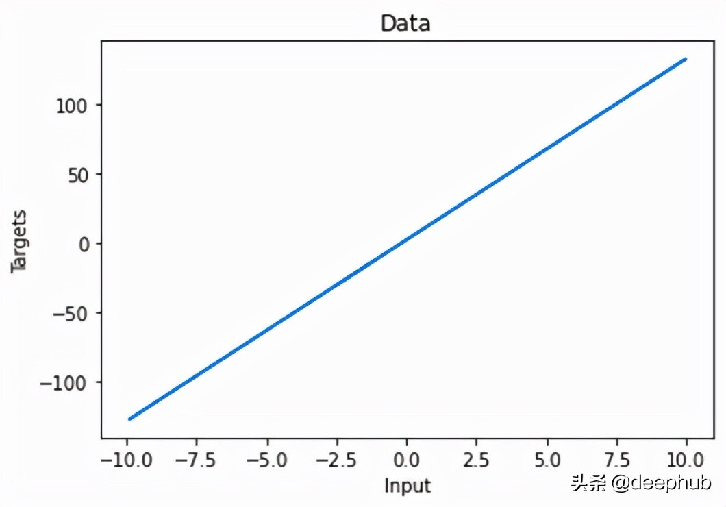
讓我們繪制生成的數據。
- # Plot x and targets
- plt.plot(x,targets)
- # Add labels to x axis and y axis
- plt.ylabel('Targets')
- plt.xlabel('Input')
- # Add title to the graph
- plt.title('Data')
- # Show the plot
- plt.show()
圖 3 顯示了這種線性關系:
對于模型訓練,我們將從參數的一些初始值開始。 它們是從給定范圍內的隨機均勻分布生成的。 您可以看到這些值與真實值相差甚遠。
- np.random.seed(42)
- # We will initialize the weights and biases randomly within a small initial range.
- # init_range is the variable that will measure that.
- init_range = 0.1
- # Weights are of size k x m, where k is the number of input variables and m is the number of output variables
- # In our case, the weights matrix is 1 x 1, since there is only one input (x) and one output (y)
- weights = np.random.uniform(low=-init_range, high=init_range, size=(1, 1))
- # Biases are of size 1 since there is only 1 output. The bias is a scalar.
- biases = np.random.uniform(low=-init_range, high=init_range, size=1)
- # Print the weights to get a sense of how they were initialized.
- # You can see that they are far from the actual values.
- print (weights)
- print (biases)
- [[-0.02509198]]
- [0.09014286]
我們還為我們的訓練設置了學習率。 我們選擇了 0.02 的值。 這里可以通過嘗試不同的值來探索性能。 我們有了數據,初始化了參數,并設置了學習率,已準備好開始訓練過程。 我們通過將 epochs 設置為 100 來迭代數據。在每個 epoch 中,我們使用初始參數來計算新輸出并將它們與實際輸出進行比較。 損失函數用于根據前面提到的梯度下降規則更新參數。 新更新的參數用于下一次迭代。 這個過程會不斷重復,直到達到 epoch 數。 可以有其他停止訓練的標準,但我們今天不討論它。
- # Set some small learning rate
- # 0.02 is going to work quite well for our example. Once again, you can play around with it.
- # It is HIGHLY recommended that you play around with it.
- learning_rate = 0.02
- # We iterate over our training dataset 100 times. That works well with a learning rate of 0.02.
- # We call these iteration epochs.
- # Let us define a variable to store the loss of each epoch.
- losses = []
- for i in range (100):
- # This is the linear model: y = xw + b equation
- outputs = np.dot(x,weights) + biases
- # The deltas are the differences between the outputs and the targets
- # Note that deltas here is a vector 1000 x 1
- deltas = outputs - targets
- # We are considering the L2-norm loss as our loss function (regression problem), but divided by 2.
- # Moreover, we further divide it by the number of observations to take the mean of the L2-norm.
- loss = np.sum(deltas ** 2) / 2 / observations
- # We print the loss function value at each step so we can observe whether it is decreasing as desired.
- print (loss)
- # Add the loss to the list
- losses.append(loss)
- # Another small trick is to scale the deltas the same way as the loss function
- # In this way our learning rate is independent of the number of samples (observations).
- # Again, this doesn't change anything in principle, it simply makes it easier to pick a single learning rate
- # that can remain the same if we change the number of training samples (observations).
- deltas_scaled = deltas / observations
- # Finally, we must apply the gradient descent update rules.
- # The weights are 1 x 1, learning rate is 1 x 1 (scalar), inputs are 1000 x 1, and deltas_scaled are 1000 x 1
- # We must transpose the inputs so that we get an allowed operation.
- weights = weights - learning_rate * np.dot(x.T,deltas_scaled)
- biases = biases - learning_rate * np.sum(deltas_scaled)
- # The weights are updated in a linear algebraic way (a matrix minus another matrix)
- # The biases, however, are just a single number here, so we must transform the deltas into a scalar.
- # The two lines are both consistent with the gradient descent methodology.
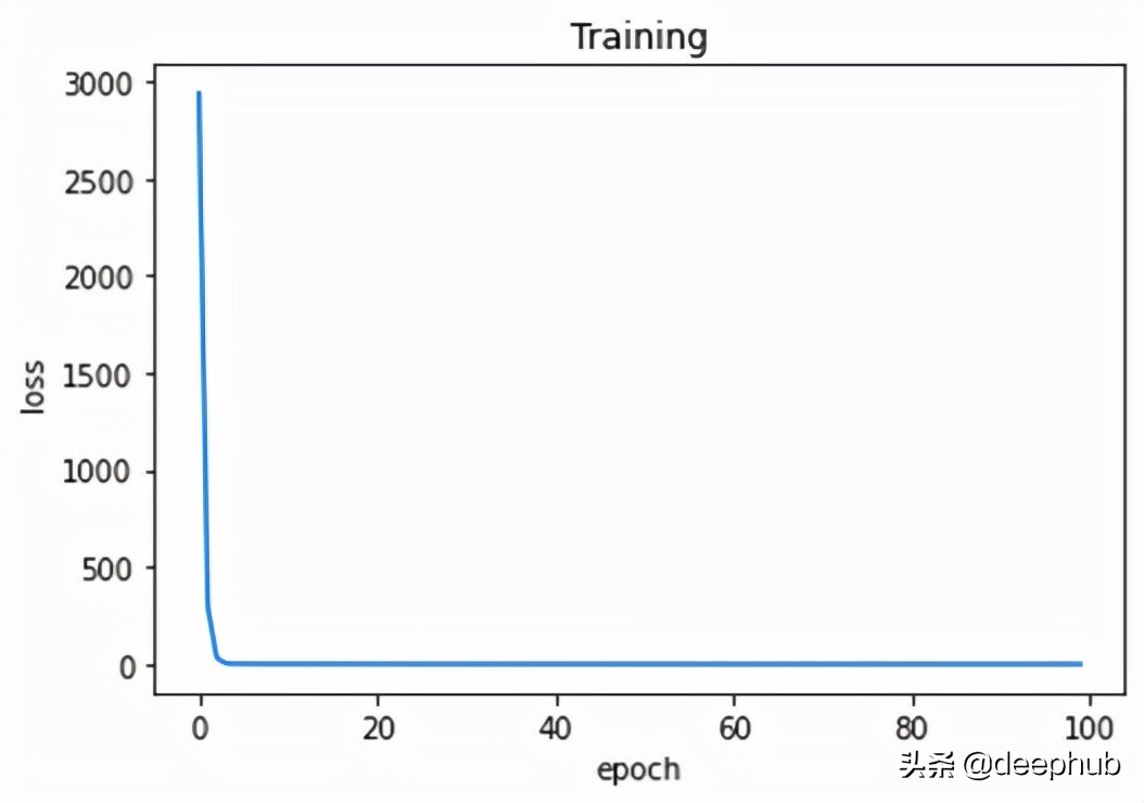
我們可以觀察每個輪次的訓練損失。
- # Plot epochs and losses
- plt.plot(range(100),losses)
- # Add labels to x axis and y axis
- plt.ylabel('loss')
- plt.xlabel('epoch')
- # Add title to the graph
- plt.title('Training')
- # Show the plot
- # The curve is decreasing in each epoch, which is what we need
- # After several epochs, we can see that the curve is flattened.
- # This means the algorithm has converged and hence there are no significant updates
- # or changes in the weights or biases.
- plt.show()
正如我們從圖 4 中看到的,損失在每個 epoch 中都在減少。 這意味著模型越來越接近參數的真實值。 幾個 epoch 后,損失沒有顯著變化。 這意味著模型已經收斂并且參數不再更新(或者更新非常小)。
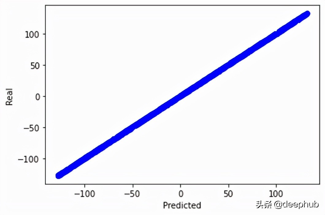
此外,我們可以通過繪制實際輸出和預測輸出來驗證我們的模型在找到真實關系方面的指標。
- # We print the real and predicted targets in order to see if they have a linear relationship.
- # There is almost a total match between the real targets and predicted targets.
- # This is a good signal of the success of our machine learning model.
- plt.plot(outputs,targets, 'bo')
- plt.xlabel('Predicted')
- plt.ylabel('Real')
- plt.show()
- # We print the weights and the biases, so we can see if they have converged to what we wanted.
- # We know that the real weight is 13 and the bias is 2
- print (weights, biases)
這將生成如圖 5 所示的圖形。我們甚至可以打印最后一個 epoch 之后的參數值。 顯然,更新后的參數與實際參數非常接近。
- [[13.09844702]] [1.73587336]
Numpy 實現線性回歸模型就是這樣。
Keras 實現
我們首先導入必要的模塊。 TensorFlow 是這個實現的核心。 它是構建模型所必需的。 Keras 是 TensorFlow 的抽象,以便于使用。
- # Numpy is needed to generate the data
- import numpy as np
- # Matplotlib is needed for visualization
- import matplotlib.pyplot as plt
- # TensorFlow is needed for model build
- import tensorflow as tf
為了生成數據(特征和目標),我們使用了 Numpy 中生成數據的代碼。 我們添加了一行來將 Numpy 數組保存在一個文件中,以防我們想將它們與其他模型一起使用(可能不需要,但添加它不會有什么壞處)。
- np.savez('TF_intro', inputs=x, targets=targets)
Keras 有一個 Sequential 的類。 它用于堆疊創建模型的層。 由于我們只有一個特征和輸出,因此我們將只有一個稱為密集層的層。 這一層負責線性變換 (W*X +B),這是我們想要的模型。 該層有一個稱為神經元的計算單元用于輸出計算,因為它是一個回歸模型。 對于內核(權重)和偏置初始化,我們在給定范圍內應用了均勻隨機分布(與 Numpy 中相同,但是在層內指定)。
- # Declare a variable where we will store the input size of our model
- # It should be equal to the number of variables you have
- input_size = 1
- # Declare the output size of the model
- # It should be equal to the number of outputs you've got (for regressions that's usually 1)
- output_size = 1
- # Outline the model
- # We lay out the model in 'Sequential'
- # Note that there are no calculations involved - we are just describing our network
- model = tf.keras.Sequential([
- # Each 'layer' is listed here
- # The method 'Dense' indicates, our mathematical operation to be (xw + b)
- tf.keras.layers.Input(shape=(input_size , )),
- tf.keras.layers.Dense(output_size,
- # there are extra arguments you can include to customize your model
- # in our case we are just trying to create a solution that is
- # as close as possible to our NumPy model
- # kernel here is just another name for the weight parameter
- kernel_initializer=tf.random_uniform_initializer(minval=-0.1, maxval=0.1),
- bias_initializer=tf.random_uniform_initializer(minval=-0.1, maxval=0.1)
- )
- ])
- # Print the structure of the model
- model.summary()
為了訓練模型,keras提供 fit 的方法可以完成這項工作。 因此,我們首先加載數據,指定特征和標簽,并設置輪次。 在訓練模型之前,我們通過選擇合適的優化器和損失函數來配置模型。 這就是 compile 的作用。 我們使用了學習率為 0.02(與之前相同)的隨機梯度下降,損失是均方誤差。
- # Load the training data from the NPZ
- training_data = np.load('TF_intro.npz')
- # We can also define a custom optimizer, where we can specify the learning rate
- custom_optimizer = tf.keras.optimizers.SGD(learning_rate=0.02)
- # 'compile' is the place where you select and indicate the optimizers and the loss
- # Our loss here is the mean square error
- model.compile(optimizer=custom_optimizer, loss='mse')
- # finally we fit the model, indicating the inputs and targets
- # if they are not otherwise specified the number of epochs will be 1 (a single epoch of training),
- # so the number of epochs is 'kind of' mandatory, too
- # we can play around with verbose; we prefer verbose=2
- model.fit(training_data['inputs'], training_data['targets'], epochs=100, verbose=2)
我們可以在訓練期間監控每個 epoch 的損失,看看是否一切正常。 訓練完成后,我們可以打印模型的參數。 顯然,模型已經收斂了與實際值非常接近的參數值。
- # Extracting the weights and biases is achieved quite easily
- model.layers[0].get_weights()
- # We can save the weights and biases in separate variables for easier examination
- # Note that there can be hundreds or thousands of them!
- weights = model.layers[0].get_weights()[0]
- bias = model.layers[0].get_weights()[1]
- bias,weights
- (array([1.9999999], dtype=float32), array([[13.1]], dtype=float32))
當您構建具有數千個參數和不同層的復雜模型時,TensorFlow 可以為您節省大量精力和代碼行。 由于模型太簡單,這里并沒有顯示keras的優勢。
PyTorch 實現
我們導入 Torch。這是必須的,因為它將用于創建模型。
- # Numpy is needed for data generation
- import numpy as np
- # Pytorch is needed for model build
- import torch
數據生成部分未顯示,因為它與前面使用的代碼相同。 但是Torch 只處理張量(torch.Tensor)。所以需要將特征和目標數組都轉換為張量。 最后,從這兩個張量創建一個張量數據集。
- # TensorDataset is needed to prepare the training data in form of tensors
- from torch.utils.data import TensorDataset
- # To run the model on either the CPU or GPU (if available)
- device = 'cuda' if torch.cuda.is_available() else 'cpu'
- # Since torch deals with tensors, we convert the numpy arrays into torch tensors
- x_tensor = torch.from_numpy(x).float()
- y_tensor = torch.from_numpy(targets).float()
- # Combine the feature tensor and target tensor into torch dataset
- train_data = TensorDataset(x_tensor , y_tensor)
模型的創建很簡單。 與keras類似,Sequential 類用于創建層堆棧。 我們只有一個線性層(keras叫密集層),一個輸入和一個輸出。 模型的參數使用定義的函數隨機初始化。 為了配置模型,我們設置了學習率、損失函數和優化器。 還有其他參數需要設置,這里不做介紹。
- # Initialize the seed to make the code reproducible
- torch.manual_seed(42)
- # This function is for model's parameters initialization
- def init_weights(m):
- if isinstance(m, torch.nn.Linear):
- torch.nn.init.uniform_(m.weight , a = -0.1 , b = 0.1)
- torch.nn.init.uniform_(m.bias , a = -0.1 , b = 0.1)
- # Define the model using Sequential class
- # It contains only a single linear layer with one input and one output
- model = torch.nn.Sequential(torch.nn.Linear(1 , 1)).to(device)
- # Initialize the model's parameters using the defined function from above
- model.apply(init_weights)
- # Print the model's parameters
- print(model.state_dict())
- # Specify the learning rate
- lr = 0.02
- # The loss function is the mean squared error
- loss_fn = torch.nn.MSELoss(reduction = 'mean')
- # The optimizer is the stochastic gradient descent with a certain learning rate
- optimizer = torch.optim.SGD(model.parameters() , lr = lr)
我們將使用小批量梯度下降訓練模型。 DataLoader 負責從訓練數據集創建批次。 訓練類似于keras的實現,但使用不同的語法。 關于 Torch訓練有幾點補充:
1- 模型和批次必須在同一設備(CPU 或 GPU)上。
2- 模型必須設置為訓練模式。
3- 始終記住在每個 epoch 之后將梯度歸零以防止累積(對 epoch 的梯度求和),這會導致錯誤的值。
- # DataLoader is needed for data batching
- from torch.utils.data import DataLoader
- # Training dataset is converted into batches of size 16 samples each.
- # Shuffling is enabled for randomizing the data
- train_loader = DataLoader(train_data , batch_size = 16 , shuffle = True)
- # A function for training the model
- # It is a function of a function (How fancy)
- def make_train_step(model , optimizer , loss_fn):
- def train_step(x , y):
- # Set the model to training mode
- model.train()
- # Feedforward the model with the data (features) to obtain the predictions
- yhat = model(x)
- # Calculate the loss based on the predicted and actual targets
- loss = loss_fn(y , yhat)
- # Perform the backpropagation to find the gradients
- loss.backward()
- # Update the parameters with the calculated gradients
- optimizer.step()
- # Set the gradients to zero to prevent accumulation
- optimizer.zero_grad()
- return loss.item()
- return train_step
- # Call the training function
- train_step = make_train_step(model , optimizer , loss_fn)
- # To store the loss of each epoch
- losses = []
- # Set the epochs to 100
- epochs = 100
- # Run the training function in each epoch on the batches of the data
- # This is why we have two for loops
- # Outer loop for epochs
- # Inner loop for iterating through the training data batches
- for epoch in range(epochs):
- # To accumulate the losses of all batches within a single epoch
- batch_loss = 0
- for x_batch , y_batch in train_loader:
- x_batch = x_batch.to(device)
- y_batch = y_batch.to(device)
- loss = train_step(x_batch , y_batch)
- batch_loss = batch_loss + loss
- # 63 is not a magic number. It is the number of batches in the training set
- # we have 1000 samples and the batch size is 16 (defined in the DataLoader)
- # 1000/16 = 63
- epoch_loss = batch_loss / 63
- losses.append(epoch_loss)
- # Print the parameters after the training is done
- print(model.state_dict())
- OrderedDict([('0.weight', tensor([[13.0287]], device='cuda:0')), ('0.bias', tensor([2.0096], device='cuda:0'))])
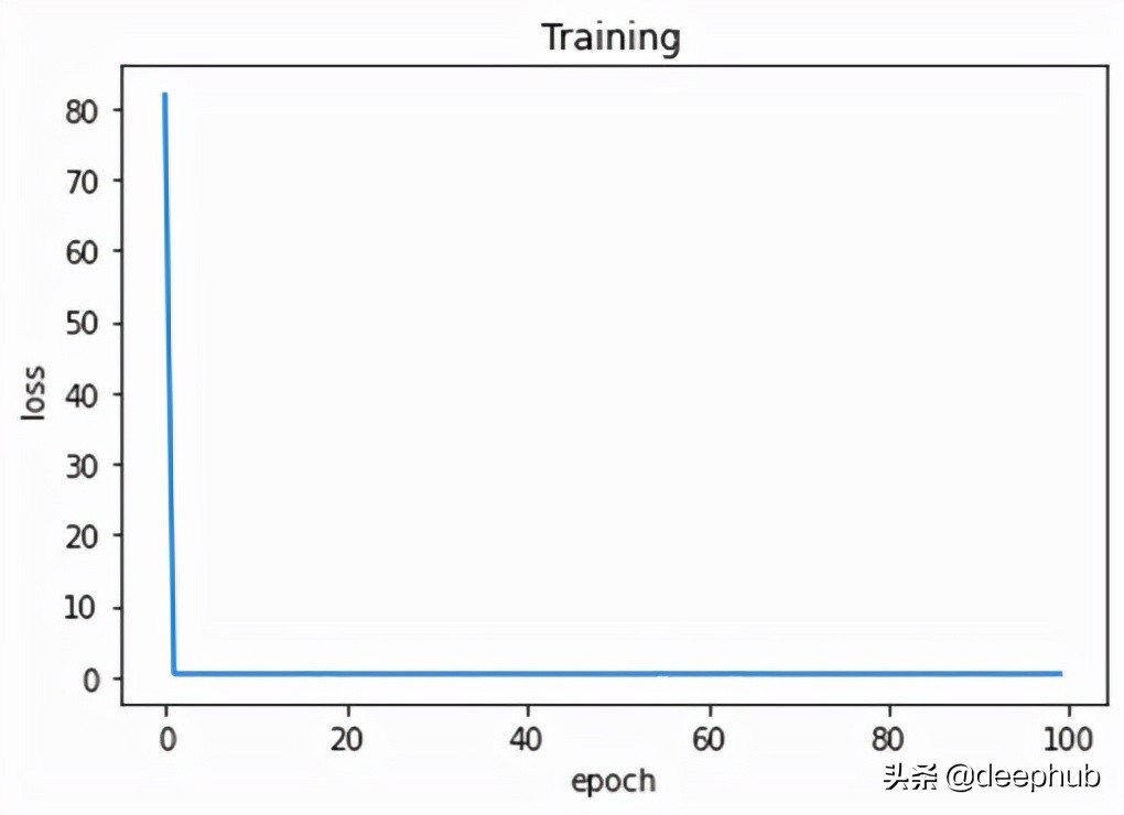
作為最后一步,我們可以繪制 epoch 上的訓練損失以觀察模型的性能。 如圖 6 所示。
完成。 讓我們總結一下到目前為止我們學到的東西。
總結
線性回歸被認為是最容易實現和解釋的機器學習模型之一。 在本文中,我們使用 Python 中的三個不同的流行模塊實現了線性回歸。 還有其他模塊可用于創建。 例如,Scikitlearn。