最強總結,必會的十大機器學習算法!
1.線性回歸
線性回歸(Linear Regression)是最基本的回歸分析方法之一,旨在通過線性模型來描述因變量(目標變量)與自變量(特征變量)之間的關系。
線性回歸假設目標變量 y 與特征變量 X 之間呈現線性關系,模型公式為:
其中:

 圖片
圖片
線性回歸的目標是找到最優的回歸系數 ,使得預測值與實際值之間的差異最小。
# Importing Libraries
import numpy as np
from sklearn.linear_model import LinearRegression
import matplotlib.pyplot as plt

# ensures that the random numbers generated are the same every time the code runs.
np.random.seed(0)

#creates an array of 100 random numbers between 0 and 1.
X = np.random.rand(100, 1)

#generates the target variable y using the linear relationship y = 2 + 3*X plus some random noise. This mimics real-world data that might not fit perfectly on a line.
y = 2 + 3 * X + np.random.rand(100, 1)

# Create and fit the model
model = LinearRegression()
# fit means it calculates the best-fitting line through the data points.
model.fit(X, y)

# Make predictions
X_test = np.array([[0], [1]])   #creates a test set with two points: 0 and 1
y_pred = model.predict(X_test)   # uses the fitted model to predict the y values for X_test


# Plot the results
plt.figure(figsize=(10, 6))
plt.scatter(X, y, color='b', label='Data points')
plt.plot(X_test, y_pred, color='r', label='Regression line')
plt.legend()
plt.xlabel('X')
plt.ylabel('y')
plt.title('Linear Regression Example\nimage by ishaangupta1201')
plt.show()


print(f"Intercept: {model.intercept_[0]:.2f}")
print(f"Coefficient: {model.coef_[0][0]:.2f}")
2.邏輯回歸
邏輯回歸(Logistic Regression)雖然帶有“回歸”之名,但其實是一種廣義線性模型,常用于二分類問題。
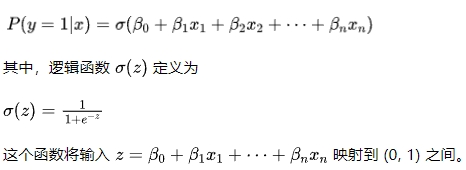
邏輯回歸的核心思想是通過邏輯函數(Logistic Function),將線性回歸模型的輸出映射到區間 (0, 1) 上,來表示事件發生的概率。
對于一個給定的輸入特征 x,模型預測為:
 圖片
圖片
import numpy as np
from sklearn.linear_model import LogisticRegression

# Sample data: hours studied and pass/fail outcome
hours_studied = np.array([1, 2, 3, 4, 5, 6, 7, 8, 9, 10]).reshape(-1, 1)
outcome = np.array([0, 0, 0, 0, 0, 1, 1, 1, 1, 1])

# Create and train the model
model = LogisticRegression()
model.fit(hours_studied, outcome)

# This results in an array of predicted binary outcomes (0 or 1).
predicted_outcome = model.predict(hours_studied)

# This results in an array where each sub-array contains two probabilities: the probability of failing and the probability of passing.
predicted_probabilities = model.predict_proba(hours_studied)

print("Predicted Outcomes:", predicted_outcome)
print("Predicted Probabilities:", predicted_probabilities)
3. 決策樹
決策樹是一種基于樹結構的監督學習算法,可用于分類和回歸任務。
決策樹模型由節點和邊組成,每個節點表示一個特征或決策,邊代表根據特征值分裂數據的方式。樹的葉子節點對應最終的預測結果。
決策樹通過遞歸地選擇最佳的特征進行分裂,直到所有數據被準確分類或滿足某些停止條件。常用的分裂標準包括信息增益(Information Gain)和基尼指數(Gini Index)。
 圖片
圖片
from sklearn.tree import DecisionTreeClassifier, plot_tree
from sklearn.datasets import load_iris
from sklearn.model_selection import train_test_split
from sklearn.metrics import accuracy_score, classification_report

# Load the iris dataset
iris = load_iris()
X, y = iris.data, iris.target

# splits the data into training and testing sets. 30% of the data is used for testing (test_size=0.3), and the rest for training. random_state=42 ensures the split is reproducible.
X_train, X_test, y_train, y_test = train_test_split(X, y, test_size=0.3, random_state=42)

# creates a decision tree classifier with a maximum depth of 3 levels and a fixed random state for reproducibility.
model = DecisionTreeClassifier(max_depth=3, random_state=42)
model.fit(X_train, y_train)

# Make predictions
y_pred = model.predict(X_test)

# Evaluate the model
accuracy = accuracy_score(y_test, y_pred)  #calculates the accuracy of the model’s predictions.
print(f"Accuracy: {accuracy:.2f}")
print("\nClassification Report:")
print(classification_report(y_test, y_pred, target_names=iris.target_names))

# Visualize the tree
plt.figure(figsize=(20,10))
plot_tree(model, feature_names=iris.feature_names, class_names=iris.target_names, filled=True, rounded=True)
plt.show()
4.支持向量機
支持向量機 (SVM) 是一種監督學習算法,可用于分類或回歸問題。
SVM 的核心思想是找到一個超平面,將數據點分成不同的類,并且這個超平面能夠最大化兩類數據點之間的間隔(Margin)。
超平面
超平面是一個能夠將不同類別的數據點分開的決策邊界。
在二維空間中,超平面就是一條直線;在三維空間中,超平面是一個平面;而在更高維空間中,超平面是一個維度比空間低一維的幾何對象。
形式上,在 n 維空間中,超平面可以表示為。

在 SVM 中,超平面用于將不同類別的數據點分開,即將正類數據點與負類數據點分隔開。
支持向量
支持向量是指在分類問題中,距離超平面最近的數據點。
這些點在 SVM 中起著關鍵作用,因為它們直接影響到超平面的位置和方向。
間隔
間隔(Margin)是指超平面到最近的支持向量的距離。
最大間隔
最大間隔是指支持向量機在尋找超平面的過程中,選擇能夠使正類和負類數據點之間的間隔最大化的那個超平面。
 圖片
圖片
from sklearn.datasets import load_wine
from sklearn.svm import SVC
from sklearn.model_selection import train_test_split

# Load the wine dataset
X, y = load_wine(return_X_y=True)

# Split the data into training and testing sets
X_train, X_test, y_train, y_test = train_test_split(X, y, test_size=0.2, random_state=42)

# Create and train the model
model = SVC(kernel='linear', random_state=42)
model.fit(X_train, y_train)

# Make predictions
y_pred = model.predict(X_test)

print("Predictions:", y_pred)
5.樸素貝葉斯
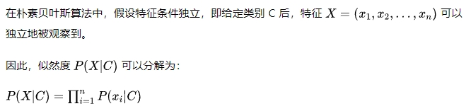
樸素貝葉斯是一種基于貝葉斯定理的簡單而強大的分類算法,廣泛用于文本分類、垃圾郵件過濾等問題。
其核心思想是假設所有特征之間相互獨立,并通過計算每個類別的后驗概率來進行分類。
貝葉斯定理定義為

from sklearn.datasets import load_digits
from sklearn.naive_bayes import GaussianNB
from sklearn.model_selection import train_test_split

# Load the digits dataset
X, y = load_digits(return_X_y=True)

# Split the data into training and testing sets
X_train, X_test, y_train, y_test = train_test_split(X, y, test_size=0.2, random_state=42)

# Create and train the model
model = GaussianNB()
model.fit(X_train, y_train)

# Make predictions
y_pred = model.predict(X_test)

print("Predictions:", y_pred)
6.KNN
K-Nearest Neighbors (KNN) 是一種簡單且直觀的監督學習算法,通常用于分類和回歸任務。
它的基本思想是:給定一個新的數據點,算法通過查看其最近的 K 個鄰居來決定這個點所屬的類別(分類)或預測其值(回歸)。
KNN 不需要顯式的訓練過程,而是直接在預測時利用整個訓練數據集。
 圖片
圖片
算法步驟
- 步驟1
選擇參數 K,即最近鄰居的數量。 - 步驟2
計算新數據點與訓練數據集中所有點之間的距離。
常用的距離度量包括歐氏距離、曼哈頓距離、切比雪夫距離等。 - 步驟3
根據計算出的距離,找出距離最近的 K 個點。 - 步驟4
對于分類問題,通過對這 K 個點的類別進行投票,選擇得票最多的類別作為新數據點的預測類別。
對于回歸問題,計算這 K 個點的平均值,作為新數據點的預測值。 - 步驟5
返回預測結果。
from sklearn.datasets import load_iris
from sklearn.neighbors import KNeighborsClassifier
from sklearn.model_selection import train_test_split

# Load the iris dataset
X, y = load_iris(return_X_y=True)

# Split the data into training and testing sets
X_train, X_test, y_train, y_test = train_test_split(X, y, test_size=0.2, random_state=42)

# Create and train the model
model = KNeighborsClassifier(n_neighbors=3)
model.fit(X_train, y_train)

# Make predictions
y_pred = model.predict(X_test)

print("Predictions:", y_pred)
7.K-Means
K-Means 是一種流行的無監督學習算法,主要用于聚類分析。
它的目標是將數據集分成 K 個簇,使得每個簇中的數據點與簇中心的距離最小。
算法通過迭代優化來達到最優的聚類效果。
 圖片
圖片
算法步驟
- 步驟1
初始化 K 個簇中心(質心)。可以隨機選擇數據集中的 K 個點作為初始質心。 - 步驟2
對于數據集中每個數據點,將其分配到與其距離最近的質心所在的簇。 - 步驟3
重新計算每個簇的質心,即簇中所有點的平均值。 - 步驟4
重復步驟2和步驟3,直到質心不再變化或變化量小于設定的閾值。
from sklearn.datasets import make_blobs
from sklearn.cluster import KMeans

# Create a synthetic dataset
X, _ = make_blobs(n_samples=100, centers=3, n_features=2, random_state=42)

# Create and train the model
model = KMeans(n_clusters=3, random_state=42)
model.fit(X)

# Predict the clusters
labels = model.predict(X)

print("Cluster labels:", labels)
8.隨機森林
隨機森林 (Random Forest) 是一種集成學習方法,主要用于分類和回歸任務。
它通過結合多個決策樹的預測結果來提高模型的泛化能力和魯棒性。
隨機森林的核心思想是通過引入隨機性來構建多個不同的決策樹模型,然后對這些模型的預測結果進行投票或平均,從而獲得最終的預測結果。
 圖片
圖片
算法步驟
- 步驟1
從訓練數據集中隨機抽取多個子樣本(使用有放回的抽樣方法,即Bootstrap抽樣),每個子樣本用于訓練一個決策樹。 - 步驟2
對于每個決策樹,在構建過程中,節點的劃分使用隨機選擇的一部分特征,而不是全部特征。 - 步驟3
每棵樹獨立生長,直到其無法進一步分裂,或者達到了某個預設的停止條件(如樹的最大深度)。 - 步驟4
對于分類任務,最終的預測結果由所有樹的投票結果決定(多數投票法);對于回歸任務,預測結果為所有樹的預測值的平均值。
from sklearn.datasets import load_breast_cancer
from sklearn.ensemble import RandomForestClassifier
from sklearn.model_selection import train_test_split

# Load the breast cancer dataset
X, y = load_breast_cancer(return_X_y=True)

# Split the data into training and testing sets
X_train, X_test, y_train, y_test = train_test_split(X, y, test_size=0.2, random_state=42)

# Create and train the model
model = RandomForestClassifier(random_state=42)
model.fit(X_train, y_train)

# Make predictions
y_pred = model.predict(X_test)

print("Predictions:", y_pred)
9.PCA
主成分分析 (PCA) 是一種用于數據降維的統計技術。
其主要目的是通過將數據從高維空間映射到一個低維空間中,保留盡可能多的原始數據的方差。
這對于數據預處理和可視化非常有用,尤其是在處理具有大量特征的數據集時。
PCA 的核心思想是找到數據中的“主成分”(即那些方差最大且相互正交的方向),并沿著這些方向投影數據,從而降低數據的維度。
通過這種方式,PCA 可以在減少數據維度的同時盡可能保留數據的整體信息。
from sklearn.datasets import load_digits
from sklearn.decomposition import PCA

# Load the digits dataset
X, y = load_digits(return_X_y=True)

# Apply PCA to reduce the number of features
pca = PCA(n_compnotallow=2)
X_reduced = pca.fit_transform(X)

print("Reduced feature set shape:", X_reduced.shape)
10.xgboost
XGBoost(Extreme Gradient Boosting)是一種基于梯度提升框架的高效、靈活的機器學習算法。
它是梯度提升決策樹 (GBDT) 的一種實現,具有更高的性能和更好的可擴展性,常被用來處理結構化或表格數據,并在各種數據競賽中表現優異。
XGBoost 的核心思想是通過迭代構建多個決策樹,每個新樹都嘗試糾正前一個樹的誤差。最終的預測結果是所有樹的預測結果的加權和。
 圖片
圖片
import xgboost as xgb
from sklearn.datasets import load_breast_cancer
from sklearn.model_selection import train_test_split

# Load the breast cancer dataset
X, y = load_breast_cancer(return_X_y=True)

# Split the data into training and testing sets
X_train, X_test, y_train, y_test = train_test_split(X, y, test_size=0.2, random_state=42)

# Create and train the model
model = xgb.XGBClassifier(random_state=42)
model.fit(X_train, y_train)

# Make predictions
y_pred = model.predict(X_test)

print("Predictions:", y_pred)