被GPT4o的讀圖能力震撼到了
I will send you 11 pictures and please explain what is in the picture and guess its usage, give your answer in English and then translate into Chinese
我會發給你11張圖片,請解釋圖片中有什么并猜測其用途,用英語給出你的答案,然后翻譯成中文
?? Sure, go ahead and upload the pictures one by one. I'll describe each picture and guess its usage, then provide the translation in Chinese for you.
當然可以,一張一張上傳照片。我將描述每個圖片并猜測其用法,然后為您提供中文翻譯。
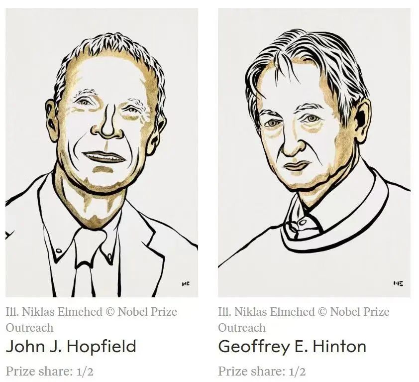
this is picture number 1
?? This image features two illustrated portraits accompanied by names and credits. The left figure is John J. Hopfield, and the right figure is Geoffrey E. Hinton. Their illustrations likely signify their contributions and recognition in a professional or academic field. The text mentions a "Prize share," suggesting they might be recipients of a significant award or honor, such as a Nobel Prize.
這張圖片展示了兩幅插畫肖像及其名字和版權信息。左邊的圖像代表John J. Hopfield,右邊的是Geoffrey E. Hinton。這些插畫可能象征著他們在某個專業或學術領域的貢獻和認可。文中提到的“獎項份額”暗示他們可能是某個重要獎項或榮譽(例如諾貝爾獎)的獲得者。

this is picture number 2
?? This image displays a famous equation from statistical mechanics, S=k?logW, which is associated with Ludwig Eduard Boltzmann, given the year 1877. This equation relates the entropy (S) of a system to the number of possible microstates (W), with k being the Boltzmann constant. It is a fundamental principle in the field of thermodynamics and statistical mechanics.
這張圖片展示了一條著名的統計力學方程式 S=k?logW,并與Ludwig Eduard Boltzmann 相關,年份為1877。這個方程式將一個系統的熵(S)與可能的微觀狀態數量(W)聯系起來,其中 k是玻爾茲曼常數。這是熱力學和統計力學領域的基本原理。
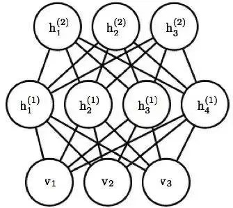
this is picture number 3
?? This image depicts a diagram of a neural network, specifically a restricted Boltzmann machine (RBM). The network consists of visible units (v1,v2,v3) and hidden units (h1(1),h2(1),h3(1),h4(1) in the first layer, and h1(2),h2(2),h3(2) in the second layer). The connections between these units illustrate how the input data (visible units) are connected to the hidden units in a hierarchical manner, common in machine learning and artificial intelligence applications.
這張圖片展示了一個神經網絡的圖示,特別是一個受限玻爾茲曼機(RBM)。網絡包括可見單元 (v1,v2,v3) 和隱藏單元 (h1(1),h2(1),h3(1),h4(1)在第一層,h1(2),h2(2),h3(2) 在第二層)。這些單元之間的連接展示了輸入數據(可見單元)如何以分層方式連接到隱藏單元,這在機器學習和人工智能應用中很常見。
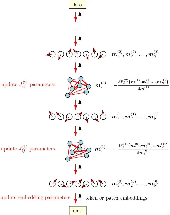
this is number 4
?? This image appears to illustrate a process in a machine learning or neural network training workflow. It details the sequence of updating parameters (Jij) in different layers and embeddings, from data input to calculating loss. The process starts with the data, which goes through an embedding layer to tokenize or create patch embeddings. These embeddings pass through various layers where parameters are updated, and computations are performed. The end goal is to minimize the loss.
這張圖片似乎展示了機器學習或神經網絡訓練流程中的某個過程。它詳細描述了從數據輸入到計算損失的各層參數(Jij)更新和嵌入的順序。該過程始于數據,通過嵌入層進行標記或創建補丁嵌入。這些嵌入通過各層,其中參數得到更新,計算得以進行。最終目標是最小化損失。
ising model is used to explain transformer in picture number 4, could you add more your explaination of this picture
在第4張圖片中,對變壓器的解釋使用了伊辛模型,你能對這張圖片進行更多的解釋嗎
?? Sure, I'll expand on the explanation with a focus on the Ising model and how it relates to transformers in the context of the image.
This image illustrates the application of the Ising model to explain the workings of a transformer, a type of neural network architecture commonly used in natural language processing and other machine learning tasks. The Ising model, traditionally used in statistical mechanics to represent magnetic systems, is adapted here to illustrate how parameters and interactions in the model can represent and process data through different layers of the transformer.
1.Data Input and Embeddings (bottom layer):
- The process begins with the input data, which is tokenized or split into patches.
- These tokens or patches are converted into embeddings, which serve as the input features for the model.
2.Update Embedding Parameters:
- The embeddings are passed through multiple layers, where their respective parameters are updated iteratively.
- In each layer, the embeddings interact with each other, similar to the interaction between spins in the Ising model.
3.First Hidden Layer ( mi(1) ):
- The first set of hidden units mi(1) is computed based on the interactions (analogous to spin interactions in the Ising model).
- The parameters Jij(1) are then updated, which can be viewed as adjusting the weights of the connections between neurons.
4.Second Hidden Layer ( mi(2) ):
- The process continues to the next hidden layer mi(2) with updated parameters Jij(2).
- This hierarchical interaction reflects how information is progressively processed and refined at each layer, akin to energy state updates in the Ising model.
5.Loss Calculation (top layer):
- The final outputs are used to compute the loss, indicating the difference between the model's prediction and the actual target.
- The loss value guides the adjustments to the parameters during training, aiming to minimize errors and improve accuracy.
In summary, this image uses the Ising model as a metaphor to illustrate the complex interactions and parameter updates within a transformer model. The analogy helps to conceptualize the dynamics of data processing through layers of neural networks, emphasizing the iterative optimization and hierarchical structure.
這張圖片使用伊辛模型來解釋變壓器(Transformer)的工作原理,這是一種常用于自然語言處理和其他機器學習任務的神經網絡架構。傳統上用于統計力學中表示磁系統的伊辛模型在這里被改編來說明模型中的參數和交互如何通過變壓器的不同層來表示和處理數據。
1.數據輸入和嵌入(底層):
- 過程從數據輸入開始,這些數據被標記化或分割成補丁。
- 這些標記或補丁被轉換為嵌入,作為模型的輸入特征。
2.更新嵌入參數:
- 嵌入通過多個層,每一層的參數都會被迭代更新。
- 在每一層中,嵌入彼此交互,類似于伊辛模型中的自旋交互。
3.第一隱藏層 (mi(1) ):
- 計算第一組隱藏單元 mi(1),基于交互(類似于伊辛模型中的自旋交互)。
- 參數 Jij(1) 隨后更新,這可以看作是調整神經元之間連接的權重。
4.第二隱藏層 (mi(2) ):
- 過程繼續到下一隱藏層 mi(2),更新參數Jij(2)。
- 這種層次交互反映了信息在每一層中逐步處理和精煉,就像伊辛模型中的能量狀態更新一樣。
5.損失計算(頂層):
- 最終輸出用于計算損失,指出模型預測與實際目標之間的差異。
- 損失值引導訓練期間參數的調整,旨在最小化錯誤并提高準確性。
總之,這張圖片使用伊辛模型作為比喻來說明變壓器模型內部的復雜交互和參數更新。這種類比有助于概念化通過神經網絡層的數據處理動態,強調迭代優化和層次結構。
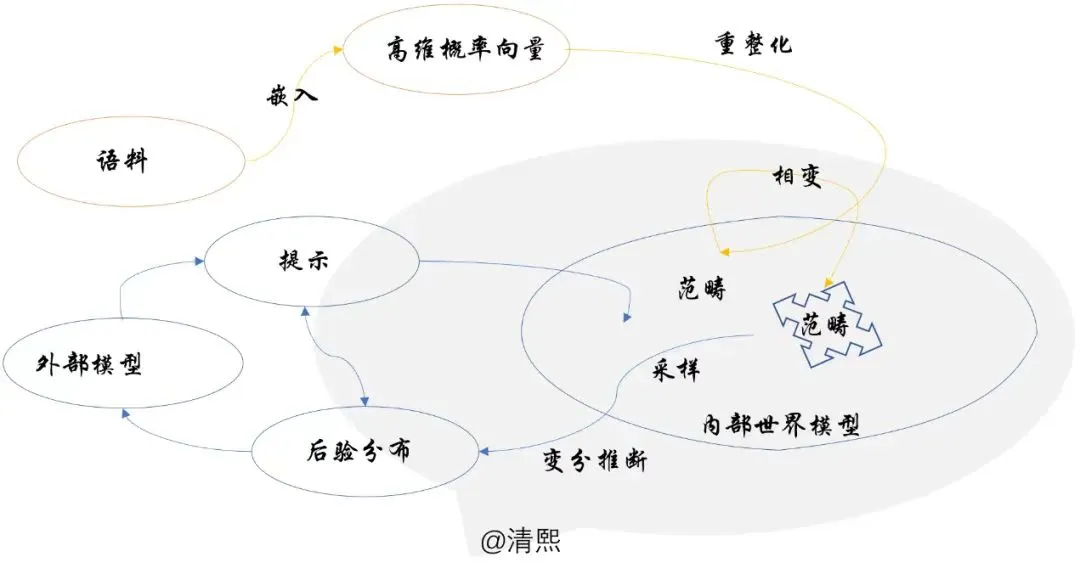
this is picture number 5
?? This image contains a flowchart with various interconnected nodes and directional arrows, indicating a process or a conceptual framework likely related to machine learning or data processing. The nodes are labeled in Chinese, suggesting steps or components within the process. Here is a breakdown of the flowchart:
?語料 (Corpus): The starting point, likely representing the raw linguistic data.
?嵌入 (Embedding): The corpus is embedded into high-dimensional vectors.
?高維概率向量 (High-dimensional probability vectors): These vectors are then reorganized (重整化) or transformed (相變).
?范疇 (Category): The process involves categorization and interaction with an "internal world model" (內部世界模型).
?采樣 (Sampling): Sampling is a crucial step within categorization.
?變分推斷 (Variational inference): Used for probabilistic and statistical inference from the data.
?后驗分布 (Posterior distribution): The results feed into the posterior distribution for further analysis.
?外部模型 (External model): Interacts with the process; external model information might be used for prompting (提示) further actions.
This process integrates statistical modeling, embedding, and inference techniques, indicating a comprehensive approach to analyzing and processing data.
這張圖片包含一個流程圖,有多個相互連接的節點和方向箭頭,表示一個過程或概念框架,可能與機器學習或數據處理相關。節點上的標簽是中文,暗示了該過程中的步驟或組件。以下是流程圖的細分:
?語料:起點,可能代表原始的語言數據。
?嵌入:語料被嵌入到高維向量中。
?高維概率向量:這些向量然后被重整化或相變。
?范疇:過程中涉及分類和與“內部世界模型”的交互。
?采樣:采樣是分類中的一個關鍵步驟。
?變分推斷:用于從數據中進行概率統計推斷。
?后驗分布:結果反饋到后驗分布中進一步分析。
?外部模型:與過程有交互;外部模型信息可能用于提示進一步的行動。
這個過程結合了統計建模、嵌入和推斷技術,表明是一個綜合的方法來分析和處理數據。
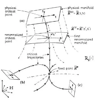
this is picture number 6
?? This image depicts a conceptual diagram that seems to explain a process related to renormalization in physics. Here is a breakdown of the main components:
1.Physical Critical Point:
- Represents the starting critical point in a physical system, likely within the context of phase transitions or critical phenomena.
2.Renormalized Critical Point:
- Shows the adjusted or "renormalized" critical point after applying some transformation or renormalization procedure, which simplifies the system while preserving essential properties.
3.Manifolds:
- Depicts different levels of physical ( H(0) ) and renormalized manifolds ( H(1) ), which are spaces upon which physical parameters lie.
4.Critical Trajectories:
- Arrows indicate the paths or trajectories that a system follows as it evolves from the physical critical point towards fixed points under renormalization transformations.
5.Fixed Point ( H? ):
- Represents a stable state where the system remains invariant under the renormalization transformations. It's a crucial concept in understanding critical behavior in systems.
6.Renormalization Operator (Rb):
- Likely represents the operator or function applied during the renormalization procedure to scale the system parameters.
This diagram is a visual tool to explain renormalization, a technique used in theoretical physics to study behaviors of systems at different scales, especially near critical points.
這張圖片展示了一個概念圖,似乎解釋了物理學中重整化相關的過程。以下是主要組成部分的細分:
1.物理臨界點:
- 代表物理系統中的起始臨界點,可能與相變或臨界現象有關。
2.重整化臨界點:
- 顯示在應用某種轉換或重整化過程后的調整或“重整化”臨界點,這簡化了系統但保留了基本特性。
3.流形:
- 描繪了物理流形( H(0) )和重整化后流形( H(1) )的不同層次,這是物理參數所在的空間。
4.臨界軌跡:
- 箭頭表示系統從物理臨界點向重整化轉換下的不動點演變的路徑或軌跡。
5.不動點( H? ):
- 代表在重整化轉換下保持不變的穩定狀態。這是理解系統在臨界行為中的重要概念。
6.重整化算子(Rb):
- 可能代表重整化過程中應用于縮放系統參數的算子或函數。
這個圖表是解釋重整化的視覺工具,重整化是一種在理論物理學中用于研究系統在不同尺度上行為的技術,特別是在臨界點附近。
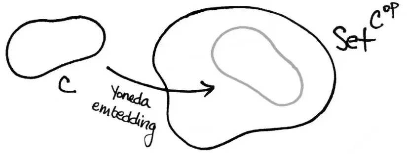
this is number 7
??This image represents a conceptual diagram related to category theory in mathematics. It illustrates the Yoneda embedding, an essential concept in category theory.
?C:
Represents a category, which is a collection of objects and morphisms (arrows) between them, satisfying certain properties.
?Set^C^op:
Denotes the category of contravariant functors from the category C to the category of sets (Set). This essentially maps objects and morphisms in a way that reverses the direction of morphisms.
?Yoneda Embedding:
The arrow indicates the Yoneda embedding, which maps an object in category C to a functor in the category Set^C^op. This embedding provides a way to represent objects of C within a functor category of presheaves, facilitating the study of C through its functor properties.
This embedding is a powerful tool in category theory, allowing category C to be understood and analyzed through the functors it represents.
這張圖片展示了一個與數學中的范疇理論相關的概念圖,說明了一個重要的概念——Yoneda嵌入。
?C:
代表一個范疇,這是滿足某些性質的對象和態射(箭頭)的集合。
?Set^C^op:
表示從范疇 C到集合范疇(Set)的反變函子范疇。這本質上是以反向映射對象和態射的方式進行映射。
?Yoneda嵌入:
箭頭表示Yoneda嵌入,它將范疇 C中的對象映射到范疇 Set^C^op 中的函子。這種嵌入提供了一種通過預層函子類別來表示C的對象的方法,從而便于通過它的函子性質來研究 C。
這種嵌入在范疇理論中是一個強有力的工具,使得可以通過它所表示的函子來理解和分析范疇 C。
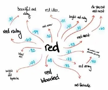
and number 8
?? This image appears to be a mind map centered around the word "red." It includes various phrases and concepts associated with "red," each linked with arrows and accompanied by numerical values, which likely represent some form of correlation, similarity score, or strength of association. Here are some of the connections depicted:
?"beautiful red ruby" with a score of .71
?"red idea" with a score of .01
?"bright red ruby" with a score of .47
?"do you eat red meat" with a score of .60
?"red meat" with a score of .53
?"the warm and passionate song" with a score of .20
?"red army" with a score of .72
?"red playdate" with a score of .36
?"red blooded" with a score of .68
?"bright red lipstick" with a score of .44
?"blood red" with a score of .82
?"red ruby" with a score of .67
Each phrase or concept extends from the central word "red," representing its various associations in different contexts, possibly aiding in studies of semantics, cognitive linguistics, or marketing analysis.
這張圖片似乎是一個圍繞“紅色”一詞的思維導圖。它包括與“紅色”相關的各種短語和概念,每個短語和數字值相關聯,這些數字可能表示某種形式的相關性、相似度分數或關聯強度。以下是其中一些連接:
?"beautiful red ruby" ,分數 .71
?"red idea" ,分數 .01
?"bright red ruby" ,分數 .47
?"do you eat red meat" ,分數 .60
?"red meat" ,分數 .53
?"the warm and passionate song" ,分數 .20
?"red army" ,分數 .72
?"red playdate" ,分數 .36
?"red blooded" ,分數 .68
?"bright red lipstick" ,分數 .44
?"blood red" ,分數 .82
?"red ruby" ,分數 .67
每個短語或概念都延伸自中心詞“紅色”,代表其在不同背景下的各種關聯,這可能有助于語義學研究、認知語言學或市場分析。

number 9
?? This image contains a mathematical equation that appears to come from the field of machine learning, particularly related to neural networks and attention mechanisms.
The equation on the left-hand side:

And the equation on the right-hand side:

Here's a breakdown of the components:
?x: Input data or feature vector.
?p: Positional encoding or additional feature vector.
?Q: Weight matrix.
?d: Dimensionality or scaling factor.
?QQ?: Possibly a self-attention matrix or another transformation related to the attention mechanism.
?softmax: A function that normalizes the input into a probability distribution.
In the context of transformers, this equation is likely part of the self-attention mechanism, which helps the model weigh the importance of different parts of the input sequence. The scaling factor 1/d is commonly used to prevent the dot products from growing too large, which the softmax function then normalizes to produce attention weights.
這張圖片包含一個數學方程,似乎來自機器學習領域,特別是與神經網絡和注意力機制相關的部分。
方程左邊:
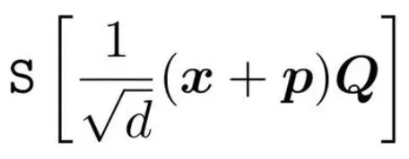
方程右邊:

以下是組成部分的細分:
?x:輸入數據或特征向量。
?p:位置編碼或額外的特征向量。
?Q:權重矩陣。
?d:維度或縮放因子。
?QQ?:可能是自注意力矩陣或與注意力機制相關的其他變換。
?softmax:一個將輸入歸一化為概率分布的函數。
在變壓器的上下文中,這個方程可能是自注意力機制的一部分,幫助模型權衡輸入序列不同部分的重要性。縮放因子 1/d常用于防止點積變得太大,之后 softmax 函數則將其歸一化以生成注意力權重。
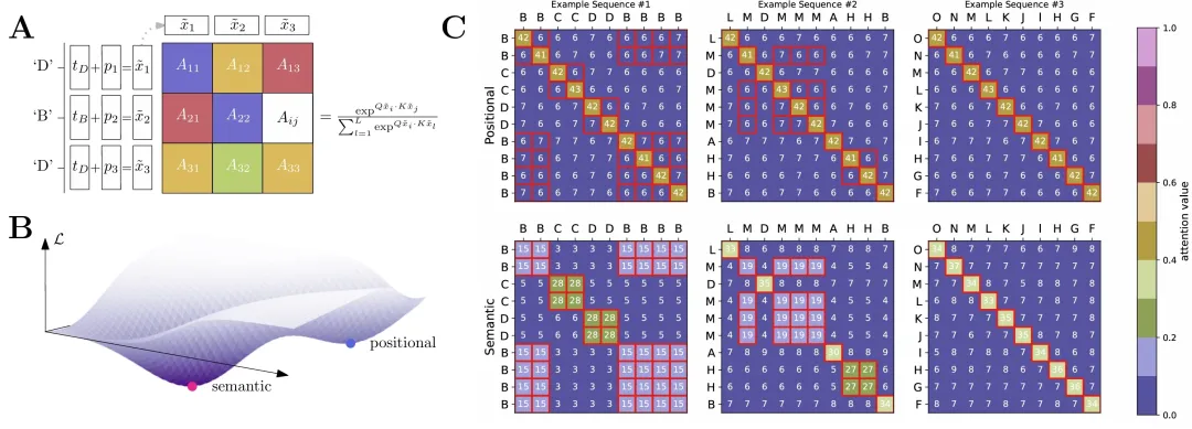
number 10
?? This image is divided into three main sections labeled A, B, and C, each contributing to the explanation of some data analysis or machine learning concept related to attention mechanisms.
Section A
Illustration of Attention Mechanism:
?Inputs and Summation:
?Inputs (D, B, D) are transformed through positional encoding ( p) and temporal encoding ( t), resulting in encoded vectors x~1,x~2,x~3.
?The resulting encoded inputs are used to create an attention map represented by matrix Aij.
?Scaled Dot-Product Attention:
?The formula at the right side shows how the attention weights Aij are calculated. These are usually based on the scaled dot-product of the encoder outputs.
?Each element Aij in the attention map is computed using the softmax function of the scaled dot-product of the query Q and key K vectors.
Section B
Semantic and Positional Interplay:
?This section visualizes the interplay between positional and semantic information in a 3D plot.
?Positional and Semantic: Axes indicating two different types of information carried by the input tokens.
?Loss Surface: The plot likely represents a loss landscape ( L ) which changes based on the balance of positional and semantic information.
Section C
Attention Maps for Example Sequences:
?Heatmaps for Different Example Sequences:
?Three sets of heatmaps (Example Sequence #1, #2, #3) shown using blue, U-shaped structures, with color-coded values indicating attention strength.
?Sequences such as letters or numbers run along the axes of each heatmap.
?Attention Values: Colormaps to the right indicate the attention value of normalized scores (where higher attention values indicate a stronger focus by the model on those elements).
?Positional vs. Semantic Representation:
?Positional Heatmaps: Display how attention is distributed purely based on the positional context of the tokens.
?Semantic Heatmaps: Show attention distribution considering the semantic context.
Summary
?Attention Mechanism in Transformers: The sections collectively help illustrate how attention mechanisms in transformer models balance positional and semantic information across sequences.
?Visualization Techniques: Both 3D plots and heatmaps provide insight into transformation and influence of input data, primarily with a focus on enhancing interpretability for language models.
這張圖片分為三部分,A,B 和 C,各自說明了與注意力機制相關的數據分析或機器學習概念。
部分 A
注意力機制圖解:
?輸入和加法:
?輸入(D,B,D)經過位置編碼( p )和時間編碼( t )后,生成編碼向量x~1,x~2,x~3。
?這些編碼的輸入用于創建一個表示為矩陣 Aij的注意力圖。
?縮放點積注意力:
?右側的公式展示了如何計算注意力權重 Aij,通常基于編碼器輸出的縮放點積。
?注意力圖中的每個元素 Aij是通過查詢向量 Q 和鍵向量 K 的縮放點積的軟最大值函數計算的。
部分 B
語義和位置之間的交互:
?這一部分通過3D圖展示了位置信息與語義信息之間的交互。
?位置信息 和 語義信息:表示輸入 tokens 中兩種不同信息類型的坐標軸。
?損失曲面:圖中顯示的可能是損失景觀 (L),基于位置和語義信息的平衡改變的曲面。
部分 C
示例序列的注意力圖:
?不同示例序列的熱力圖:
?三組熱力圖(Example Sequence #1, #2, #3)在藍色 U 形結構中展示,顏色編碼的數值指示注意力強度。
?每個熱力圖的坐標軸上排列著字母或數字序列。
?注意力數值:右側的顏色圖表示歸一化分數的注意力數值(注意力數值越高表示模型對這些元素的關注度越強)。
?位置與語義表示:
?位置熱力圖:顯示注意力如何僅基于 tokens 的位置上下文進行分布。
?語義熱力圖:顯示考慮語義上下文的注意力分布。
總結
?變壓器中的注意力機制:這些部分共同說明了變壓器模型中的注意力機制如何在序列中平衡位置和語義信息。
?可視化技術:3D圖和熱力圖提供了輸入數據的轉化和影響的見解,主要是為了增強語言模型的可解釋性。
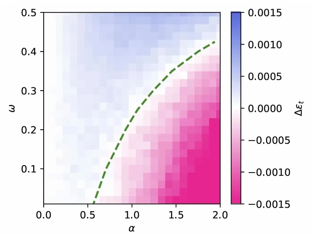
number 11
?? This image is a heatmap that represents data across two variables, αα and ωω, with a color gradient indicating the value of a third variable Δ?t. Here’s a breakdown of the elements:
1.Axes:
X-axis (α): Represents a variable range from 0 to 2.
Y-axis (ω): Represents another variable range from 0 to 0.5.
2.Color Gradient:
The color bar to the right shows the range of Δ?t values, with blue indicating lower values and pink/red indicating higher values. The gradient ranges from approximately -0.0015 to 0.0015.
3.Heatmap:
The heatmap itself is a visual representation of Δ?t values for the corresponding α and ω pairs. Each pixel's color reflects the value of Δ?t at that point.
4.Dashed Line:
?A green dashed line suggests a boundary or threshold within the data, indicating a region where there's a significant change in behavior or a phase transition.
This heatmap can be used to analyze how Δ?t varies with α and ω, helping to identify patterns, trends, or critical points in the data.
這張圖片是一個熱圖,表示在兩個變量 α 和 ω上的數據,顏色漸變指示第三個變量 Δ?t的值。以下是元素的詳細信息:
1.軸線:
X軸 (α):表示從0到2的變量范圍。
Y軸 (ω):表示從0到0.5的另一個變量范圍。
2.顏色漸變:
右側的顏色條顯示 Δ?t值的范圍,藍色表示較低值,粉紅或紅色表示較高值。漸變范圍大約從 -0.0015 到 0.0015。
3.熱圖:
熱圖本身是 Δ?t值針對相應的α和ω對的可視化表示。每個像素的顏色反映該點 Δ?t的值。
4.虛線:
綠色的虛線暗示數據中的邊界或閾值,表明某個區域內有顯著變化或相變的行為。
該熱圖可用于分析 Δ?t隨α和ω的變化,以幫助識別數據中的模式、趨勢或臨界點。
本文轉載自 ??清熙??,作者: 王慶法


