[[217972]]

關于房價，一直都是全民熱議的話題，畢竟不少人終其一生都在為之奮斗。

房地產的泡沫究竟有多大不得而知？今天我們拋開泡沫，回歸房屋最本質的內容，來分析一下房價的影響因素究竟是什么？

1、導入數據

import numpy as np 
 
import pandas as pd 
 
import matplotlib.pyplot as plt 
 
import seaborn as sn 
 
import missingno as msno 
 
%matplotlib inline 
 
train = pd.read_csv('train.csv',index_col=0)  
 
#導入訓練集 
 
test = pd.read_csv('test.csv',index_col=0)  
 
#導入測試集 
 
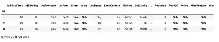
train.head(3) 
 
print('train訓練集缺失數據分布圖') 
 
msno.matrix(train) 
 
print('test測試集缺失數據分布圖') 
 
msno.matrix(test) 

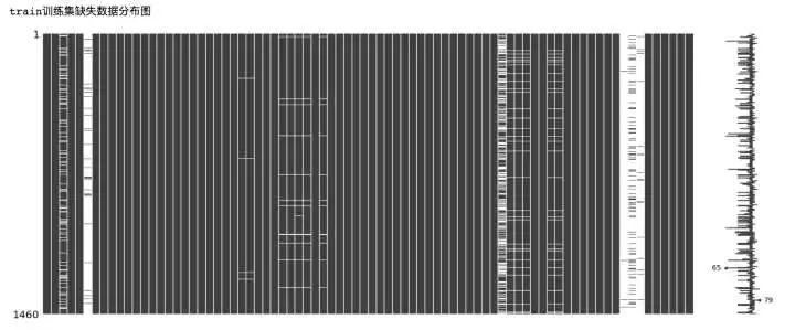
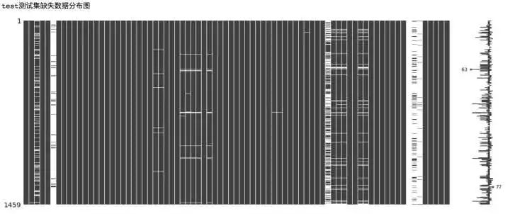
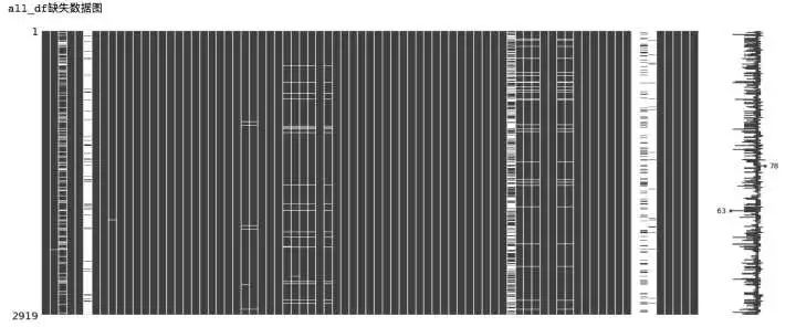
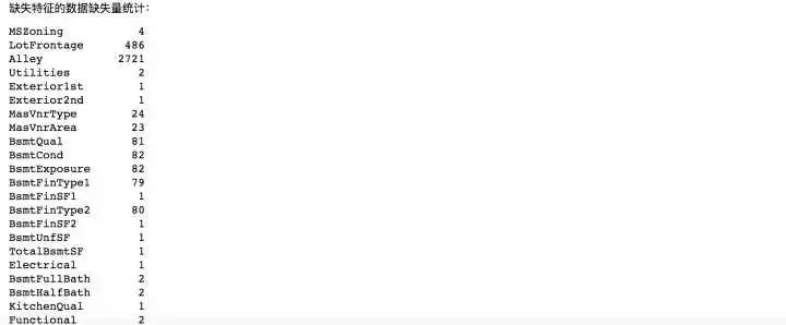
從上面的數據缺失可視化圖中可以看出，部分特征的數據缺失十分嚴重，下面我們來對特征的缺失數量進行統計。

2、目標Y值分析 

##分割Y和X數據 
 
y=train['SalePrice'] 
 
#看一下y的值分布 
 
prices = pd.DataFrame({'price':y,'log(price+1)':np.log1p(y)}) 
 
prices.hist() 

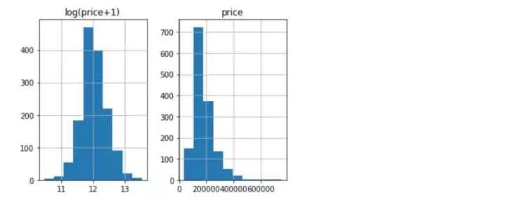
觀察目標變量y的分布和取對數后的分布看，取完對數后更傾向于符合正太分布，故我們對y進行對數轉化。 

y = np.log1p(y) #+1的目的是防止對數轉化后的值無意義 

3、合并數據 缺失處理 

#合并訓練特征和測試集 
 
all_df = pd.concat((X,test),axis=0) 
 
print('all_df缺失數據圖') 
 
msno.matrix(all_df) 
 
#定義缺失統計函數 
 
def show_missing(feature): 
 
    missing = feature.columns[feature.isnull().any()].tolist()     
 
    return  missing 
 
print('缺失特征的數據缺失量統計：') 
 
all_df[show_missing(all_df)].isnull().sum() 
 
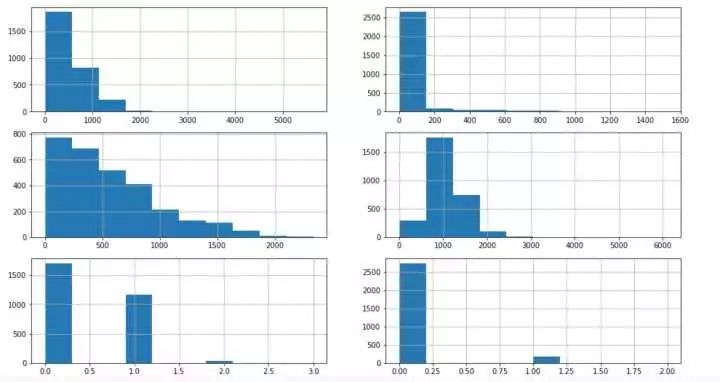
#先處理numeric數值型數據 
 
#挨個兒看一下分布 
 
fig,axs = plt.subplots(3,2,figsize=(16,9)) 
 
all_df['BsmtFinSF1'].hist(ax = axs[0,0])#眾數填充 
 
all_df['BsmtFinSF2'].hist(ax = axs[0,1])#眾數 
 
all_df['BsmtUnfSF'].hist(ax =  axs[1,0])#中位數 
 
all_df['TotalBsmtSF'].hist(ax = axs[1,1])#均值填充 
 
all_df['BsmtFullBath'].hist(ax = axs[2,0])#眾數 
 
all_df['BsmtHalfBath'].hist(ax = axs[2,1])#眾數 
 
#lotfrontage用均值填充 
 
mean_lotfrontage = all_df.LotFrontage.mean() 
 
all_df.LotFrontage.hist() 
 
print('用均值填充:') 
 
cat_input(all_df,'LotFrontage',mean_lotfrontage) 
 
cat_input(all_df,'BsmtFinSF1',0.0) 
 
cat_input(all_df,'BsmtFinSF2',0.0) 
 
cat_input(all_df,'BsmtFullBath',0.0) 
 
cat_input(all_df,'BsmtHalfBath',0.0) 
 
cat_input(all_df,'BsmtUnfSF',467.00) 
 
cat_input(all_df,'TotalBsmtSF',1051.78) 
 
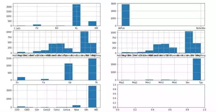
#在處理字符型，同樣，挨個看下分布 
 
fig,axs = plt.subplots(4,2,figsize=(16,9)) 
 
all_df['MSZoning'].hist(ax = axs[0,0])#眾數填充 
 
all_df['Utilities'].hist(ax = axs[0,1])#眾數 
 
all_df['Exterior1st'].hist(ax =  axs[1,0])#眾數 
 
all_df['Exterior2nd'].hist(ax = axs[1,1])#眾數填充 
 
all_df['KitchenQual'].hist(ax = axs[2,0])#眾數 
 
all_df['Functional'].hist(ax = axs[2,1])#眾數 
 
all_df['SaleType'].hist(ax = axs[3,0])#眾數 
 
cat_input(all_df,'MSZoning','RL') 
 
cat_input(all_df,'Utilities','AllPub') 
 
cat_input(all_df,'Exterior1st','VinylSd') 
 
cat_input(all_df,'Exterior2nd','VinylSd') 
 
cat_input(all_df,'KitchenQual','TA') 
 
cat_input(all_df,'Functional','Typ') 
 
cat_input(all_df,'SaleType','WD') 
 
#再看一下缺失分布 
 
msno.matrix(all_df) 

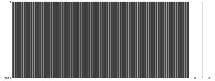
binggo，數據干凈啦！下面開始處理特征,經過上述略微復雜的處理，數據集中所有的缺失數據都已處理完畢，可以開始接下來的工作啦！

缺失處理總結：在本篇文章所使用的數據集中存在比較多的缺失，缺失數據包括數值型和字符型，處理原則主要有兩個：

一、根據繪制數據分布直方圖，觀察數據分布的狀態，采取合適的方式填充缺失數據；

二、非常重要的特征描述，認真閱讀，按照特征描述填充可以解決大部分問題。

4、特征處理

讓我們在重新仔細審視一下數據有沒有問題？仔細觀察發現MSSubClass特征實際上是分類特征，但是數據顯示是int類型，這個需要改成str。 

#觀察特征屬性發現，MSSubClass是分類特征，但是數據給的是數值型，需要對其做轉換 
 
all_df['MSSubClass']=all_df['MSSubClass'].astype(str) 
 
#將分類變量轉變成數值變量 
 
all_df = pd.get_dummies(all_df) 
 
print('分類變量轉換完成后有{}行{}列'.format(*all_df.shape))  

分類變量轉換完成后有2919行316列 

#標準化處理 
 
numeric_cols = all_df.columns[all_df.dtypes !='uint8'] 
 
#x-mean(x)/std(x) 
 
numeric_mean = all_df.loc[:,numeric_cols].mean() 
 
numeric_std = all_df.loc[:,numeric_cols].std() 
 
all_df.loc[:,numeric_cols] = (all_df.loc[:,numeric_cols]-numeric_mean)/numeric_std  

再把數據拆分到訓練集和測試集 

train_df = all_df.ix[0:1460]#訓練集 
 
test_df = all_df.ix[1461:]#測試集  

5、構建基準模型 

from sklearn import cross_validation 
 
from sklearn import linear_model 
 
from sklearn.learning_curve import learning_curve 
 
from sklearn.metrics import explained_variance_score 
 
from sklearn.grid_search import GridSearchCV 
 
from sklearn.model_selection import cross_val_score 
 
from sklearn.ensemble import RandomForestRegressor 
 
y = y.values #轉換成array數組 
 
X = train_df.values #轉換成array數組 
 
cv = cross_validation.ShuffleSplit(len(X),n_iter=3,test_size=0.2) 
 
print('嶺回歸交叉驗證結果：') 
 
for train_index,test_index in cv: 
 
    ridge = linear_model.Ridge(alpha=1).fit(X,y)     
 
   print('train_score:{0:.3f},test_score:{1:.3f}\n'.format(ridge.score(X[train_index],y[train_index]), ridge.score(X[test_index],y[test_index]))) 
 
print('隨機森林交叉驗證結果：') 
 
for train_index,test_index in cv: 
 
    rf = RandomForestRegressor().fit(X,y)     
 
    print('train_score:{0:.3f},test_score:{1:.3f}\n'.format(rf.score(X[train_index],y[train_index]), rf.score(X[test_index],y[test_index]))) 

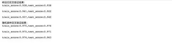
哇！好意外啊，這兩個模型的結果表現都不錯，但是隨機森林的結果似乎更好，下面來看看學習曲線情況。

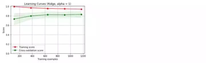
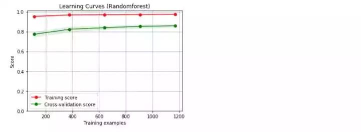
我們采用的是默認的參數，沒有調優處理，得到的兩個基準模型都存在過擬合現象。下面，我們開始著手參數的調整，希望能夠改善模型的過擬合現象。

6、參數調優

嶺回歸正則項縮放系數alpha調整 

alphas =[0.01,0.1,1,10,20,50,100,300] 
 
test_scores = [] 
 
for alp in alphas: 
 
    clf = linear_model.Ridge(alp) 
 
    test_score = -cross_val_score(clf,X,y,cv=10,scoring='neg_mean_squared_error') 
 
    test_scores.append(np.mean(test_score)) 
 
import matplotlib.pyplot as plt 
 
%matplotlib inline 
 
plt.plot(alphas,test_scores) 
 
plt.title('alpha vs test_score') 

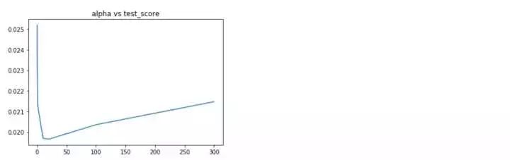
alpha在10-20附近均方誤差最小

隨機森林參數調優

隨機森林算法，本篇中主要調整三個參數：maxfeatures,maxdepth,n_estimators 

#隨機森林的深度參數 
 
max_depth=[2,4,6,8,10] 
 
test_scores_depth = [] 
 
for depth in max_depth: 
 
    clf = RandomForestRegressor(max_depth=depth) 
 
    test_score_depth = -cross_val_score(clf,X,y,cv=10,scoring='neg_mean_squared_error') 
 
    test_scores_depth.append(np.mean(test_score_depth)) 
 
#隨機森林的特征個數參數 
 
max_features =[.1, .3, .5, .7, .9, .99] 
 
test_scores_feature = [] 
 
for feature in max_features: 
 
    clf = RandomForestRegressor(max_features=feature) 
 
    test_score_feature = -cross_val_score(clf,X,y,cv=10,scoring='neg_mean_squared_error') 
 
    test_scores_feature.append(np.mean(test_score_feature)) 
 
#隨機森林的估計器個位數參數 
 
n_estimators =[10,50,100,200,500] 
 
test_scores_n = [] 
 
for n in n_estimators: 
 
    clf = RandomForestRegressor(n_estimators=n) 
 
    test_score_n = -cross_val_score(clf,X,y,cv=10,scoring='neg_mean_squared_error') 
 
    test_scores_n.append(np.mean(test_score_n)) 

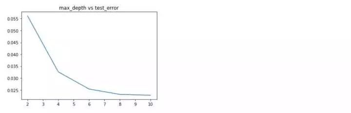
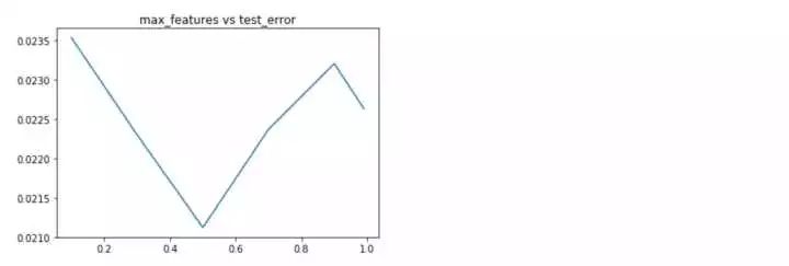
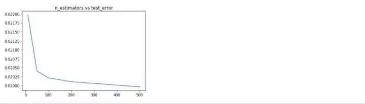
隨機森林的各項參數來看，深度位于8，選擇特征個數比例為0.5，估計器個數為500時，效果***。下面分別利用上述得到的***參數分別重新訓練，看一下學習曲線，過擬合現象是否得到緩解？

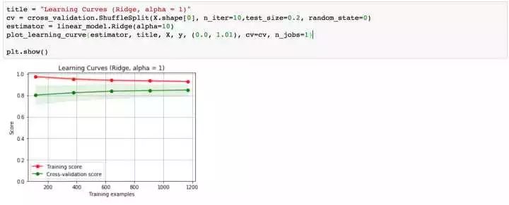
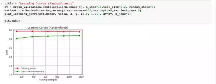
再回想一下，我們最初的基線模型學習曲線的形狀，是不是得到了一定程度的緩解？OK，下面我們采用模型融合技術，對數據進行預測。 

#預測 
 
ridge = linear_model.Ridge(alpha=10).fit(X,y) 
 
rf = RandomForestRegressor(n_estimators=500,max_depth=8,max_features=.5).fit(X,y) 
 
y_ridge = np.expm1(ridge.predict(test_df.values)) 
 
y_rf = np.expm1(rf.predict(test_df.values)) 
 
y_final = (y_ridge + y_rf)/2 

本篇房價預測的模型搭建已經完成。同樣，再梳理一邊思路：

一、本篇用到的房價數據集存在比較多的數據缺失，且分類變量十分多。在預處理階段需要將訓練集和測試集合并，進行缺失填充和one-hot獨熱變量處理，保證數據處理過程的一致性，在數據缺失填充過程中，需要綜合考慮特征的實際描述和數據的分布，選擇合適的填充方式填充；

二、為防止數據變量不統一帶來的模型準確率下降，將數值型特征進行標準化處理，數據處理完成后，按照數據合并的方式，再還原到訓練集和測試集；

三、先構建嶺回歸和隨機森林基準模型，進行三折交叉驗證，繪制學習曲線，存在明顯的過擬合現象；

四、接下來分別對兩個基準模型進行參數調優，獲得使得均方誤差最小的參數，返回到訓練集進行訓練； 

五、采用并行模型融合的方式，計算兩個模型預測結果的均值作為測試集的預測結果。