無監督學習是一類用于在數據中尋找模式的機器學習技術。無監督學習算法使用的輸入數據都是沒有標注過的，這意味著數據只給出了輸入變量(自變量 X)而沒有給出相應的輸出變量(因變量)。在無監督學習中，算法本身將發掘數據中有趣的結構。

人工智能研究的領軍人物 Yan Lecun，解釋道：無監督學習能夠自己進行學習，而不需要被顯式地告知他們所做的一切是否正確。這是實現真正的人工智能的關鍵!

監督學習 VS 無監督學習

在監督學習中，系統試圖從之前給出的示例中學習。(而在無監督學習中，系統試圖從給定的示例中直接找到模式。)因此，如果數據集被標注過了，這就是一個監督學習問題;而如果數據沒有被標注過，這就是一個無監督學習問題。

上圖是一個監督學習的例子，它使用回歸技術找到在各個特征之間的最佳擬合曲線。而在無監督學習中，根據特征對輸入數據進行劃分，并且根據數據所屬的簇進行預測。

重要的術語

• 特征：進行預測時使用的輸入變量。
• 預測值：給定一個輸入示例時的模型輸出。
• 示例：數據集中的一行。一個示例包含一個或多個特征，可能還有一個標簽。
• 標簽：特征對應的真實結果(與預測相對應)。

準備無監督學習所需的數據

在本文中，我們使用 Iris 數據集來完成初級的預測工作。這個數據集包含 150 條記錄，每條記錄由 5 個特征構成——花瓣長度、花瓣寬度、萼片長度、萼片寬度、花的類別。花的類別包含 Iris Setosa、Iris VIrginica 和 Iris Versicolor 三種。本文中向無監督算法提供了鳶尾花的四個特征，預測它屬于哪個類別。

本文使用 Python 環境下的 sklearn 庫來加載 Iris 數據集，并且使用 matplotlib 進行數據可視化。以下是用于探索數據集的代碼片段：

# Importing Modules 
from sklearn import datasets 
import matplotlib.pyplot as plt 
 
# Loading dataset 
iris_df = datasets.load_iris() 
 
# Available methods on dataset 
print(dir(iris_df)) 
 
# Features 
print(iris_df.feature_names) 
 
# Targets 
print(iris_df.target) 
 
# Target Names 
print(iris_df.target_names) 
label = {0: 'red', 1: 'blue', 2: 'green'} 
 
# Dataset Slicing 
x_axis = iris_df.data[:, 0] # Sepal Length 
y_axis = iris_df.data[:, 2] # Sepal Width 
 
# Plotting 
plt.scatter(x_axis, y_axis, c=iris_df.target) 
plt.show() 

['DESCR', 'data', 'feature_names', 'target', 'target_names'] 
['sepal length (cm)', 'sepal width (cm)', 'petal length (cm)', 'petal width (cm)'] 
[0 0 0 0 0 0 0 0 0 0 0 0 0 0 0 0 0 0 0 0 0 0 0 0 0 0 0 0 0 0 0 0 0 0 0 0 0 0 0 0 0 0 0 0 0 0 0 0 0 0 1 1 1 1 1 1 1 1 1 1 1 1 1 1 1 1 1 1 1 1 1 1 1 1 1 1 1 1 1 1 1 1 1 1 1 1 1 1 1 1 1 1 1 1 1 1 1 1 1 1 2 2 2 2 2 2 2 2 2 2 2 2 2 2 2 2 2 2 2 2 2 2 2 2 2 2 2 2 2 2 2 2 2 2 2 2 2 2 2 2 2 2 2 2 2 2 2 2 2 2] 
['setosa' 'versicolor' 'virginica'] 

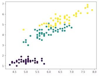
紫色：Setosa，綠色：Versicolor，黃色：Virginica

聚類分析

在聚類分析中，數據被劃分為不同的幾組。簡而言之，這一步旨在將具有相似特征的群組從整體數據中分離出來，并將它們分配到簇(cluster)中。

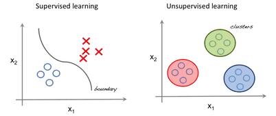
可視化示例：

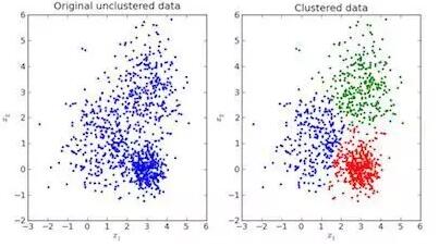
如上所示，左圖是沒有進行分類的原始數據，右圖是進行聚類之后的數據(根據數據本身的特征將其分類)。當給出一個待預測的輸入時，它會基于其特征查看自己從屬于哪一個簇，并以此為根據進行預測。

K-均值聚類的 Python 實現

K 均值是一種迭代的聚類算法，它的目標是在每次迭代中找到局部最大值。該算法要求在最初選定聚類簇的個數。由于我們知道本問題涉及到 3 種花的類別，所以我們通過將參數「n_clusters」傳遞給 K 均值模型來編寫算法，將數據分組到 3 個類別中。現在，我們隨機地將三個數據點(輸入)分到三個簇中。基于每個點之間的質心距離，下一個給定的輸入數據點將被劃分到獨立的簇中。接著，我們將重新計算所有簇的質心。

每一個簇的質心是定義結果集的特征值的集合。研究質心的特征權重可用于定性地解釋每個簇代表哪種類型的群組。

我們從 sklearn 庫中導入 K 均值模型，擬合特征并進行預測。

K 均值算法的 Python 實現：

# Importing Modules 
from sklearn import datasets 
from sklearn.cluster import KMeans 
 
# Loading dataset 
iris_df = datasets.load_iris() 
 
# Declaring Model 
model = KMeans(n_clusters=3) 
 
# Fitting Model 
model.fit(iris_df.data) 
 
# Predicitng a single input 
predicted_label = model.predict([[7.2, 3.5, 0.8, 1.6]]) 
 
# Prediction on the entire data 
all_predictions = model.predict(iris_df.data) 
 
# Printing Predictions 
print(predicted_label) 
print(all_predictions) 

[0] 
[0 0 0 0 0 0 0 0 0 0 0 0 0 0 0 0 0 0 0 0 0 0 0 0 0 0 0 0 0 0 0 0 0 0 0 0 0 0 0 0 0 0 0 0 0 0 0 0 0 0 2 2 1 2 2 2 2 2 2 2 2 2 2 2 2 2 2 2 2 2 2 2 2 2 2 2 2 1 2 2 2 2 2 2 2 2 2 2 2 2 2 2 2 2 2 2 2 2 2 2 1 2 1 1 1 1 2 1 1 1 1 1 1 2 2 1 1 1 1 2 1 2 1 2 1 1 2 2 1 1 1 1 1 2 1 1 1 1 2 1 1 1 2 1 1 1 2 1 1 2] 

層次聚類

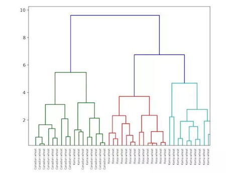
層次聚類，顧名思義，是一種能夠構建有層次的簇的算法。在這個算法的起始階段，每個數據點都是一個簇。接著，兩個最接近的簇合二為一。最終，當所有的點都被合并到一個簇中時，算法停止。

層次聚類的實現可以用 dendrogram 進行展示。接下來，我們一起來看一個糧食數據的層次聚類示例。數據集鏈接：

https://raw.githubusercontent.com/vihar/unsupervised-learning-with-python/master/seeds-less-rows.csv

1. 層次聚類的 Python 實現：

# Importing Modules 
from scipy.cluster.hierarchy import linkage, dendrogram 
import matplotlib.pyplot as plt 
import pandas as pd 
 
# Reading the DataFrame 
seeds_df = pd.read_csv( 
 "https://raw.githubusercontent.com/vihar/unsupervised-learning-with-python/master/seeds-less-rows.csv") 
 
# Remove the grain species from the DataFrame, save for later 
varieties = list(seeds_df.pop('grain_variety')) 
 
# Extract the measurements as a NumPy array 
samples = seeds_df.values 
 
""" 
Perform hierarchical clustering on samples using the 
linkage() function with the method='complete' keyword argument. 
Assign the result to mergings. 
""" 
mergings = linkage(samples, method='complete') 
 
""" 
Plot a dendrogram using the dendrogram() function on mergings, 
specifying the keyword arguments labels=varieties, leaf_rotation=90, 
and leaf_font_size=6. 
""" 
dendrogram(mergings, 
 labels=varieties, 
 leaf_rotation=90, 
 leaf_font_size=6, 
 ) 
 
plt.show() 

2. K 均值和層次聚類之間的差別

• 層次聚類不能很好地處理大數據，而 K 均值聚類可以。原因在于 K 均值算法的時間復雜度是線性的，即 O(n);而層次聚類的時間復雜度是平方級的，即 O(n2)。
• 在 K 均值聚類中，由于我們最初隨機地選擇簇，多次運行算法得到的結果可能會有較大差異。而層次聚類的結果是可以復現的。
• 研究表明，當簇的形狀為超球面(例如：二維空間中的圓、三維空間中的球)時，K 均值算法性能良好。
• K 均值算法抗噪聲數據的能力很差(對噪聲數據魯棒性較差)，而層次聚類可直接使用噪聲數據進行聚類分析。

t-SNE 聚類

這是一種可視化的無監督學習方法。t-SNE 指的是 t 分布隨機鄰居嵌入(t-distributed stochastic neighbor embedding)。它將高維空間映射到一個可視化的二維或三維空間中。具體而言，它將通過如下方式用二維或三維的數據點對高維空間的對象進行建模：以高概率用鄰近的點對相似的對象進行建模，而用相距較遠的點對不相似的對象進行建模。

用于 Iris 數據集的 t-SNE 聚類的 Python 實現：

# Importing Modules 
from sklearn import datasets 
from sklearn.manifold import TSNE 
import matplotlib.pyplot as plt 
 
# Loading dataset 
iris_df = datasets.load_iris() 
 
# Defining Model 
model = TSNE(learning_rate=100) 
 
# Fitting Model 
transformed = model.fit_transform(iris_df.data) 
 
# Plotting 2d t-Sne 
x_axis = transformed[:, 0] 
y_axis = transformed[:, 1] 
 
plt.scatter(x_axis, y_axis, c=iris_df.target) 
plt.show() 

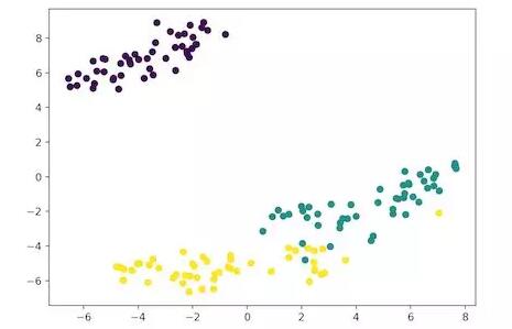
紫色：Setosa，綠色：Versicolor，黃色：Virginica

在這里，具備 4 個特征(4 維)的 Iris 數據集被轉化到二維空間，并且在二維圖像中進行展示。類似地，t-SNE 模型可用于具備 n 個特征的數據集。

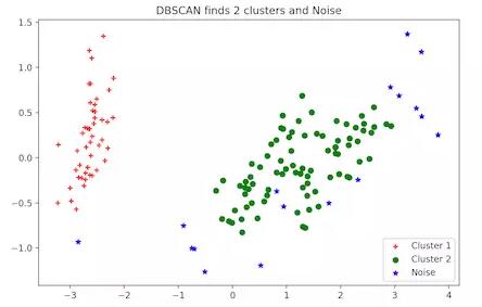
DBSCAN 聚類

DBSCAN(帶噪聲的基于密度的空間聚類方法)是一種流行的聚類算法，它被用來在預測分析中替代 K 均值算法。它并不要求輸入簇的個數才能運行。但是，你需要對其他兩個參數進行調優。

scikit-learn 的 DBSCAN 算法實現提供了缺省的「eps」和「min_samples」參數，但是在一般情況下，用戶需要對他們進行調優。參數「eps」是兩個數據點被認為在同一個近鄰中的最大距離。參數「min_samples」是一個近鄰中在同一個簇中的數據點的最小個數。

1. DBSCAN 聚類的 Python 實現：

# Importing Modules 
from sklearn.datasets import load_iris 
import matplotlib.pyplot as plt 
from sklearn.cluster import DBSCAN 
from sklearn.decomposition import PCA 
 
# Load Dataset 
iris = load_iris() 
 
# Declaring Model 
dbscan = DBSCAN() 
 
# Fitting 
dbscan.fit(iris.data) 
 
# Transoring Using PCA 
pca = PCA(n_components=2).fit(iris.data) 
pcapca_2d = pca.transform(iris.data) 
 
# Plot based on Class 
for i in range(0, pca_2d.shape[0]): 
 if dbscan.labels_[i] == 0: 
 c1 = plt.scatter(pca_2d[i, 0], pca_2d[i, 1], c='r', marker='+') 
 elif dbscan.labels_[i] == 1: 
 c2 = plt.scatter(pca_2d[i, 0], pca_2d[i, 1], c='g', marker='o') 
 elif dbscan.labels_[i] == -1: 
 c3 = plt.scatter(pca_2d[i, 0], pca_2d[i, 1], c='b', marker='*') 
 
plt.legend([c1, c2, c3], ['Cluster 1', 'Cluster 2', 'Noise']) 
plt.title('DB 

2. 更多無監督學習技術：

• 主成分分析(PCA)
• 異常檢測
• 自編碼器
• 深度信念網絡
• 赫布型學習
• 生成對抗網絡(GAN)
• 自組織映射

原文鏈接：

https://towardsdatascience.com/unsupervised-learning-with-python-173c51dc7f03

【本文是51CTO專欄機構“機器之心”的原創譯文，微信公眾號“機器之心( id: almosthuman2014)”】

戳這里，看該作者更多好文