【51CTO.com快譯】機器學習是數據科學界的王冠，而監督學習是機器學習界這頂王冠上的寶石。

背景

幾年前《哈佛商業評論》發表過一篇題為《數據科學家：21世紀最性感的工作》的文章。文章發表后，數據科學系或統計系備受大學生追捧，沉悶的數據科學家頭回被認為很性感。

對一些行業而言，數據科學家已改變了公司結構，將許多決策交給了一線員工。能夠從數據獲得實用的業務洞察力從未如此容易。

據吳恩達稱，監督學習算法為業界貢獻了大部分價值。

監督學習為什么創造如此大的業務價值不容懷疑。銀行用它來檢測信用卡欺詐，交易員根據模型做出購買決定，工廠對生產線進行過濾以查找有缺陷的零部件。

這些業務場景有兩個共同的特征：

• 二進制結果：欺詐vs不欺詐，購買vs不購買，有缺陷的vs沒有缺陷。
• 不平均的數據分布：一個多數組vs一個少數組。

正如吳恩達最近指出，小數據、穩健性和人為因素是AI項目取得成功的三大障礙。在某種程度上，一個少數組方面的罕見事件問題也是一個小數據問題：機器學習算法從多數組學到更多信息，很容易對小數據組錯誤分類。

下面是幾個事關重大的問題：

• 對于這些罕見事件，哪種機器學習方法性能更好?
• 什么度量指標?
• 有何美中不足?

本文試圖通過運用5種機器學習方法處理實際數據集來回答上述問題，附有完整的R實現代碼。

有關完整描述和原始數據集，請參閱原始數據集：https://archive.ics.uci.edu/ml/datasets/bank+marketing;有關完整的R代碼，請查看我的Github：https://github.com/LeihuaYe/Machine-Learning-Classification-for-Imbalanced-Data。

業務問題

葡萄牙一家銀行在實施一項新銀行服務(定期存款)的營銷策略，想知道哪些類型的客戶已訂購該服務，以便銀行可以在將來調整營銷策略，鎖定特定人群。數據科學家與銷售和營銷團隊合作，提出了統計解決方案，以識別未來訂戶。

R實現

以下面是模型選擇流程和R實現。

1.導入、數據清理和探索性數據分析

不妨加載并清理原始數據集。 

####load the dataset 
 
banking=read.csv(“bank-additional-full.csv”,sep =”;”,header=T)##check for missing data and make sure no missing data 
 
banking[!complete.cases(banking),]#re-code qualitative (factor) variables into numeric 
 
banking$job= recode(banking$job, “‘admin.’=1;’blue-collar’=2;’entrepreneur’=3;’housemaid’=4;’management’=5;’retired’=6;’self-employed’=7;’services’=8;’student’=9;’technician’=10;’unemployed’=11;’unknown’=12”)#recode variable again 
 
banking$marital = recode(banking$marital, “‘divorced’=1;’married’=2;’single’=3;’unknown’=4”)banking$education = recode(banking$education, “‘basic.4y’=1;’basic.6y’=2;’basic.9y’=3;’high.school’=4;’illiterate’=5;’professional.course’=6;’university.degree’=7;’unknown’=8”)banking$default = recode(banking$default, “‘no’=1;’yes’=2;’unknown’=3”)banking$housing = recode(banking$housing, “‘no’=1;’yes’=2;’unknown’=3”)banking$loan = recode(banking$loan, “‘no’=1;’yes’=2;’unknown’=3”) 
 
banking$contact = recode(banking$loan, “‘cellular’=1;’telephone’=2;”)banking$month = recode(banking$month, “‘mar’=1;’apr’=2;’may’=3;’jun’=4;’jul’=5;’aug’=6;’sep’=7;’oct’=8;’nov’=9;’dec’=10”)banking$day_of_week = recode(banking$day_of_week, “‘mon’=1;’tue’=2;’wed’=3;’thu’=4;’fri’=5;”)banking$poutcome = recode(banking$poutcome, “‘failure’=1;’nonexistent’=2;’success’=3;”)#remove variable “pdays”, b/c it has no variation 
 
banking$pdays=NULL #remove variable “pdays”, b/c itis collinear with the DV 
 
banking$duration=NULL 

清理原始數據似乎很乏味，因為我們要為缺失的變量重新編碼，并將定性變量轉換成定量變量。清理實際數據要花更長的時間。有言道“數據科學家花80%的時間來清理數據、花20%的時間來構建模型。”

下一步，不妨探究結果變量的分布。 

#EDA of the DV  
plot(banking$y,main="Plot 1: Distribution of Dependent Variable") 

圖1

由此可見，相關變量(服務訂購)并不均勻分布，“No”多過“Yes”。分布不平衡應該會發出一些警告信號，因為數據分布影響最終的統計模型。它很容易使用多數范例(majority case)開發的模型對少數范例(minority case)錯誤分類。

2. 數據分割

下一步，不妨將數據集分割成兩部分：訓練集和測試集。通常而言，我們堅持80–20分割：80%是訓練集，20%是測試集。如果是時間序列數據，我們基于90%的數據訓練模型，將剩余10%的數據作為測試數據集。 

#split the dataset into training and test sets randomly  
set.seed(1)#set seed so as to generate the same value each time we run the code#create an index to split the data: 80% training and 20% test  
index = round(nrow(banking)*0.2,digits=0)#sample randomly throughout the dataset and keep the total number equal to the value of index  
test.indices = sample(1:nrow(banking), index)#80% training set  
banking.train=banking[-test.indices,] #20% test set  
banking.test=banking[test.indices,] #Select the training set except the DV  
YTrain = banking.train$y  
XTrain = banking.train %>% select(-y)# Select the test set except the DV  
YTest = banking.test$y  
XTest = banking.test %>% select(-y) 

這里，不妨創建一個空的跟蹤記錄。 

records = matrix(NA, nrow=5, ncol=2) 
colnames(records) <- c(“train.error”,”test.error”)  
rownames(records) <- c(“Logistic”,”Tree”,”KNN”,”Random Forests”,”SVM”) 

3. 訓練模型

我們在這一節定義一個新的函數(calc_error_rate)，運用它計算每個機器學習模型的訓練和測試誤差。 

calc_error_rate <- function(predicted.value, true.value)  
{return(mean(true.value!=predicted.value))} 

如果預測的標簽與實際值不符，該函數就計算比率。

#1 邏輯回歸模型

想了解邏輯模型的簡介，不妨看看這兩篇文章：《機器學習101》(https://towardsdatascience.com/machine-learning-101-predicting-drug-use-using-logistic-regression-in-r-769be90eb03d)和《機器學習102》(https://towardsdatascience.com/machine-learning-102-logistic-regression-with-polynomial-features-98a208688c17)。

不妨添加一個邏輯模型，包括結果變量以外的所有其他變量。由于結果是二進制的，我們將模型設置為二項分布(“family-binomial”)。 

glm.fit = glm(y ~ age+factor(job)+factor(marital)+factor(education)+factor(default)+factor(housing)+factor(loan)+factor(contact)+factor(month)+factor(day_of_week)+campaign+previous+factor(poutcome)+emp.var.rate+cons.price.idx+cons.conf.idx+euribor3m+nr.employed, data=banking.train, family=binomial) 

下一步是獲得訓練誤差。由于我們預測結果的類型并采用多數規則，于是將類型設置為響應式：如果先驗概率超過或等于0.5，我們預測結果為yes，否則是no。 

prob.training = predict(glm.fit,type=”response”)banking.train_glm = banking.train %>% #select all rows of the train  
mutate(predicted.value=as.factor(ifelse(prob.training<=0.5, “no”, “yes”))) #create a new variable using mutate and set a majority rule using ifelse# get the training error  
logit_traing_error <- calc_error_rate(predicted.value=banking.train_glm$predicted.value, true.value=YTrain)# get the test error of the logistic model  
prob.test = predict(glm.fit,banking.test,type=”response”)banking.test_glm = banking.test %>% # select rows  
mutate(predicted.value2=as.factor(ifelse(prob.test<=0.5, “no”, “yes”))) # set ruleslogit_test_error <- calc_error_rate(predicted.value=banking.test_glm$predicted.value2, true.value=YTest)# write down the training and test errors of the logistic model 
records[1,] <- c(logit_traing_error,logit_test_error)#write into the first row 

#2 決策樹

若是決策樹，我們遵循交叉驗證，以識別最佳的分割節點。想大致了解決策樹，請參閱此文：https://towardsdatascience.com/decision-trees-in-machine-learning-641b9c4e8052。 

# finding the best nodes  
# the total number of rows  
nobs = nrow(banking.train)#build a DT model;  
#please refer to this document (https://www.datacamp.com/community/tutorials/decision-trees-R) for constructing a DT model  
bank_tree = tree(y~., data= banking.train,na.action = na.pass,  
control = tree.control(nobs , mincut =2, minsize = 10, mindev = 1e-3))#cross validation to prune the tree  
set.seed(3)  
cv = cv.tree(bank_tree,FUN=prune.misclass, K=10)  
cv#identify the best cv  
best.size.cv = cv$size[which.min(cv$dev)]  
best.size.cv#best = 3bank_tree.pruned<-prune.misclass(bank_tree, best=3)  
summary(bank_tree.pruned) 

交叉驗證的最佳大小是3。 

# Training and test errors of bank_tree.pruned  
pred_train = predict(bank_tree.pruned, banking.train, type=”class”)  
pred_test = predict(bank_tree.pruned, banking.test, type=”class”)# training error  
DT_training_error <- calc_error_rate(predicted.value=pred_train, true.value=YTrain)# test error  
DT_test_error <- calc_error_rate(predicted.value=pred_test, true.value=YTest)# write down the errors  
records[2,] <- c(DT_training_error,DT_test_error) 

#3 K最近鄰(KNN)

作為一種非參數方法，KNN不需要任何分布的先驗知識。簡而言之，KNN將k個數量的最近鄰分配給相關的單元。

想大致了解，不妨參閱這篇文章《R中的K最近鄰入門指南：從菜鳥到高手》：https://towardsdatascience.com/beginners-guide-to-k-nearest-neighbors-in-r-from-zero-to-hero-d92cd4074bdb。想詳細了解交叉驗證和do.chunk函數，請參閱此文：https://towardsdatascience.com/beginners-guide-to-k-nearest-neighbors-in-r-from-zero-to-hero-d92cd4074bdb。

使用交叉驗證，我們發現當k = 20時交叉驗證誤差最小。 

nfold = 10  
set.seed(1)# cut() divides the range into several intervals  
folds = seq.int(nrow(banking.train)) %>%  
cut(breaks = nfold, labels=FALSE) %>%  
sampledo.chunk <- function(chunkid, folddef, Xdat, Ydat, k){  
train = (folddef!=chunkid)# training indexXtr = Xdat[train,] # training set by the indexYtr = Ydat[train] # true label in training setXvl = Xdat[!train,] # test setYvl = Ydat[!train] # true label in test setpredYtr = knn(train = Xtr, test = Xtr, cl = Ytr, k = k) # predict training labelspredYvl = knn(train = Xtr, test = Xvl, cl = Ytr, k = k) # predict test labelsdata.frame(fold =chunkid, # k folds 
train.error = calc_error_rate(predYtr, Ytr),#training error per fold  
val.error = calc_error_rate(predYvl, Yvl)) # test error per fold  
}# set error.folds to save validation errors  
error.folds=NULL# create a sequence of data with an interval of 10  
kvec = c(1, seq(10, 50, length.out=5))set.seed(1)for (j in kvec){  
tmp = ldply(1:nfold, do.chunk, # apply do.function to each fold  
folddef=folds, Xdat=XTrain, Ydat=YTrain, k=j) # required arguments  
tmp$neighbors = j # track each value of neighbors  
error.folds = rbind(error.folds, tmp) # combine the results  
}#melt() in the package reshape2 melts wide-format data into long-format data  
errors = melt(error.folds, id.vars=c(“fold”,”neighbors”), value.name= “error”) 

隨后，不妨找到盡量減少驗證誤差的最佳K數。 

val.error.means = errors %>%  
filter(variable== “val.error” ) %>%  
group_by(neighbors, variable) %>%  
summarise_each(funs(mean), error) %>%  
ungroup() %>%  
filter(error==min(error))#the best number of neighbors =20  
numneighbor = max(val.error.means$neighbors)  
numneighbor## [20] 

遵循同一步，我們查找訓練誤差和測試誤差。 

#training error  
set.seed(20)  
pred.YTtrain = knn(train=XTrain, test=XTrain, cl=YTrain, k=20)  
knn_traing_error <- calc_error_rate(predicted.value=pred.YTtrain, true.value=YTrain)#test error =0.095set.seed(20)  
pred.YTest = knn(train=XTrain, test=XTest, cl=YTrain, k=20)  
knn_test_error <- calc_error_rate(predicted.value=pred.YTest, true.value=YTest)records[3,] <- c(knn_traing_error,knn_test_error) 

#4 隨機森林

我們遵循構建隨機森林模型的標準步驟。想大致了解隨機森林，參閱此文：https://towardsdatascience.com/understanding-random-forest-58381e0602d2。 

# build a RF model with default settings  
set.seed(1)  
RF_banking_train = randomForest(y ~ ., data=banking.train, importance=TRUE)# predicting outcome classes using training and test sets  
pred_train_RF = predict(RF_banking_train, banking.train, type=”class”)pred_test_RF = predict(RF_banking_train, banking.test, type=”class”)# training error  
RF_training_error <- calc_error_rate(predicted.value=pred_train_RF, true.value=YTrain)# test error  
RF_test_error <- calc_error_rate(predicted.value=pred_test_RF, true.value=YTest)records[4,] <- c(RF_training_error,RF_test_error) 

#5 支持向量機

同樣，我們遵循構建支持向量機的標準步驟。想大致了解該方法，請參閱此文：https://towardsdatascience.com/support-vector-machine-introduction-to-machine-learning-algorithms-934a444fca47。 

set.seed(1)  
tune.out=tune(svm, y ~., data=banking.train,  
kernel=”radial”,ranges=list(cost=c(0.1,1,10)))# find the best parameters  
summary(tune.out)$best.parameters# the best model  
best_model = tune.out$best.modelsvm_fit=svm(y~., data=banking.train,kernel=”radial”,gamma=0.05555556,cost=1,probability=TRUE)# using training/test sets to predict outcome classes  
svm_best_train = predict(svm_fit,banking.train,type=”class”)  
svm_best_test = predict(svm_fit,banking.test,type=”class”)# training error  
svm_training_error <- calc_error_rate(predicted.value=svm_best_train, true.value=YTrain)# test error  
svm_test_error <- calc_error_rate(predicted.value=svm_best_test, true.value=YTest)records[5,] <- c(svm_training_error,svm_test_error) 

4. 模型度量指標

我們已構建了遵循模型選擇過程的所有機器學習模型，并獲得了訓練誤差和測試誤差。這一節將使用一些模型的度量指標選擇最佳模型。

4.1 訓練/測試誤差

可以使用訓練/測試誤差找到最佳模型嗎?

現在不妨看看結果。

records

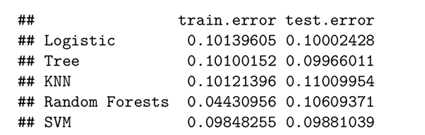
圖2

這里，隨機森林的訓練誤差最小，不過其他方法有類似的測試誤差。你可能注意到，訓練誤差和測試誤差很接近，很難說清楚哪個明顯勝出。

此外，分類精度(無論是訓練誤差還是測試誤差)都不應該是高度不平衡數據集的度量指標。這是由于數據集以多數范例為主，即使隨機猜測也會得出50%的準確性。更糟糕的是，高度精確的模型可能嚴重“處罰”少數范例。因此，不妨查看另一個度量指標：ROC曲線。

4.2受試者工作特征(ROC)曲線

ROC是一種圖形表示，顯示分類模型在所有分類閾值下有怎樣的表現。我們更喜歡比其他分類器更快逼近1的分類器。

ROC曲線在同一個圖中繪制不同閾值下的兩個參數：真陽率(True Positive Rate)和假陽率(False Positive Rate)。

TPR (Recall) = TP/(TP+FN)

FPR = FP/(TN+FP)

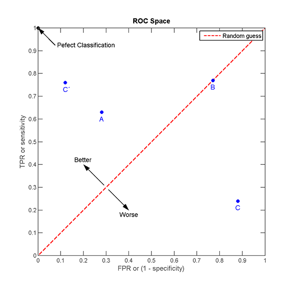
圖3

在很大程度上，ROC曲線不僅衡量分類準確度，還在TPR和FPR之間達到了很好的平衡。這是罕見事件所需要的，因為我們還想在多數范例和少數范例之間達到平衡。 

# load the library  
library(ROCR)#creating a tracking record  
Area_Under_the_Curve = matrix(NA, nrow=5, ncol=1)  
colnames(Area_Under_the_Curve) <- c(“AUC”)  
rownames(Area_Under_the_Curve) <- c(“Logistic”,”Tree”,”KNN”,”Random Forests”,”SVM”)########### logistic regression ###########  
# ROC  
prob_test <- predict(glm.fit,banking.test,type=”response”)  
pred_logit<- prediction(prob_test,banking.test$y)  
performance_logit <- performance(pred_logit,measure = “tpr”, x.measure=”fpr”)########### Decision Tree ###########  
# ROC  
pred_DT<-predict(bank_tree.pruned, banking.test,type=”vector”)  
pred_DT <- prediction(pred_DT[,2],banking.test$y)  
performance_DT <- performance(pred_DT,measure = “tpr”,x.measure= “fpr”)########### KNN ###########  
# ROC  
knn_model = knn(train=XTrain, test=XTrain, cl=YTrain, k=20,prob=TRUE)prob <- attr(knn_model, “prob”)  
prob <- 2*ifelse(knn_model == “-1”, prob,1-prob) — 1  
pred_knn <- prediction(prob, YTrain)  
performance_knn <- performance(pred_knn, “tpr”, “fpr”)########### Random Forests ###########  
# ROC  
pred_RF<-predict(RF_banking_train, banking.test,type=”prob”)  
pred_class_RF <- prediction(pred_RF[,2],banking.test$y) 
performance_RF <- performance(pred_class_RF,measure = “tpr”,x.measure= “fpr”)########### SVM ###########  
# ROC  
svm_fit_prob = predict(svm_fit,type=”prob”,newdata=banking.test,probability=TRUE)  
svm_fit_prob_ROCR = prediction(attr(svm_fit_prob,”probabilities”)[,2],banking.test$y==”yes”)  
performance_svm <- performance(svm_fit_prob_ROCR, “tpr”,”fpr”) 

不妨繪制ROC曲線。

我們添加一條直線，以顯示隨機分配的概率。我們的分類器其表現勝過隨機猜測，是不是? 

#logit  
plot(performance_logit,col=2,lwd=2,main=”ROC Curves for These Five Classification Methods”)legend(0.6, 0.6, c(‘logistic’, ‘Decision Tree’, ‘KNN’,’Random Forests’,’SVM’), 2:6)#decision tree  
plot(performance_DT,col=3,lwd=2,add=TRUE)#knn  
plot(performance_knn,col=4,lwd=2,add=TRUE)#RF  
plot(performance_RF,col=5,lwd=2,add=TRUE)# SVM  
plot(performance_svm,col=6,lwd=2,add=TRUE)abline(0,1) 

圖4

這里已分出勝負。

據ROC曲線顯示，KNN(藍色線)高于其他所有方法。

4.3 曲線下面積(AUC)

顧名思義，AUC是ROC曲線下的面積。它是直觀的AUC曲線的數學表示。AUC給出了分類器在可能的分類閾值下性能如何的合并結果。 

########### Logit ###########  
auc_logit = performance(pred_logit, “auc”)@y.values  
Area_Under_the_Curve[1,] <-c(as.numeric(auc_logit))########### Decision Tree ###########  
auc_dt = performance(pred_DT,”auc”)@y.values  
Area_Under_the_Curve[2,] <- c(as.numeric(auc_dt))########### KNN ###########  
auc_knn <- performance(pred_knn,”auc”)@y.values  
Area_Under_the_Curve[3,] <- c(as.numeric(auc_knn))########### Random Forests ###########  
auc_RF = performance(pred_class_RF,”auc”)@y.values  
Area_Under_the_Curve[4,] <- c(as.numeric(auc_RF))########### SVM ###########  
auc_svm<-performance(svm_fit_prob_ROCR,”auc”)@y.values[[1]]  
Area_Under_the_Curve[5,] <- c(as.numeric(auc_svm)) 

不妨查看AUC值。

Area_Under_the_Curve

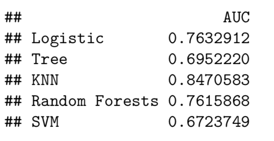
圖5

此外，KNN擁有最大的AUC值(0.847)。

結束語

我們在本文中發現KNN這個非參數分類器的表現勝過參數分類器。就度量指標而言，為罕見事件選擇ROC曲線而非分類準確度來得更合理。

原文標題：Classify A Rare Event Using 5 Machine Learning Algorithms，作者：Leihua Ye 

【51CTO譯稿，合作站點轉載請注明原文譯者和出處為51CTO.com】