5分鐘掌握Python隨機爬山算法

隨機爬山是一種優化算法。它利用隨機性作為搜索過程的一部分。這使得該算法適用于非線性目標函數,而其他局部搜索算法不能很好地運行。它也是一種局部搜索算法,這意味著它修改了單個解決方案并搜索搜索空間的相對局部區域,直到找到局部最優值為止。這意味著它適用于單峰優化問題或在應用全局優化算法后使用。
在本教程中,您將發現用于函數優化的爬山優化算法完成本教程后,您將知道:
- 爬山是用于功能優化的隨機局部搜索算法。
- 如何在Python中從頭開始實現爬山算法。
- 如何應用爬山算法并檢查算法結果。
教程概述
本教程分為三個部分:他們是:
- 爬山算法
- 爬山算法的實現
- 應用爬山算法的示例
爬山算法
隨機爬山算法是一種隨機局部搜索優化算法。它以起始點作為輸入和步長,步長是搜索空間內的距離。該算法將初始點作為當前最佳候選解決方案,并在提供的點的步長距離內生成一個新點。計算生成的點,如果它等于或好于當前點,則將其視為當前點。新點的生成使用隨機性,通常稱為隨機爬山。這意味著該算法可以跳過響應表面的顛簸,嘈雜,不連續或欺騙性區域,作為搜索的一部分。重要的是接受具有相等評估的不同點,因為它允許算法繼續探索搜索空間,例如在響應表面的平坦區域上。限制這些所謂的“橫向”移動以避免無限循環也可能是有幫助的。該過程一直持續到滿足停止條件,例如最大數量的功能評估或給定數量的功能評估內沒有改善為止。該算法之所以得名,是因為它會(隨機地)爬到響應面的山坡上,達到局部最優值。這并不意味著它只能用于最大化目標函數。這只是一個名字。實際上,通常,我們最小化功能而不是最大化它們。作為局部搜索算法,它可能會陷入局部最優狀態。然而,多次重啟可以允許算法定位全局最優。步長必須足夠大,以允許在搜索空間中找到更好的附近點,但步幅不能太大,以使搜索跳出包含局部最優值的區域。
爬山算法的實現
在撰寫本文時,SciPy庫未提供隨機爬山的實現。但是,我們可以自己實現它。首先,我們必須定義目標函數和每個輸入變量到目標函數的界限。目標函數只是一個Python函數,我們將其命名為Objective()。邊界將是一個2D數組,每個輸入變量都具有一個維度,該變量定義了變量的最小值和最大值。例如,一維目標函數和界限將定義如下:
- # objective function
- def objective(x):
- return 0
- # define range for input
- bounds = asarray([[-5.0, 5.0]])
接下來,我們可以生成初始解作為問題范圍內的隨機點,然后使用目標函數對其進行評估。
- # generate an initial point
- solution = bounds[:, 0] + rand(len(bounds)) * (bounds[:, 1] - bounds[:, 0])
- # evaluate the initial point
- solution_eval = objective(solution)
現在我們可以遍歷定義為“ n_iterations”的算法的預定義迭代次數,例如100或1,000。
- # run the hill climb
- for i in range(n_iterations):
算法迭代的第一步是采取步驟。這需要預定義的“ step_size”參數,該參數相對于搜索空間的邊界。我們將采用高斯分布的隨機步驟,其中均值是我們的當前點,標準偏差由“ step_size”定義。這意味著大約99%的步驟將在當前點的(3 * step_size)之內。
- # take a step
- candidate = solution + randn(len(bounds)) * step_size
我們不必采取這種方式。您可能希望使用0到步長之間的均勻分布。例如:
- # take a step
- candidate = solution + rand(len(bounds)) * step_size
接下來,我們需要評估具有目標函數的新候選解決方案。
- # evaluate candidate point
- candidte_eval = objective(candidate)
然后,我們需要檢查此新點的評估結果是否等于或優于當前最佳點,如果是,則用此新點替換當前最佳點。
- # check if we should keep the new point
- if candidte_eval <= solution_eval:
- # store the new point
- solution, solution_eval = candidate, candidte_eval
- # report progress
- print('>%d f(%s) = %.5f' % (i, solution, solution_eval))
就是這樣。我們可以將此爬山算法實現為可重用函數,該函數將目標函數的名稱,每個輸入變量的范圍,總迭代次數和步驟作為參數,并返回找到的最佳解決方案及其評估。
- # hill climbing local search algorithm
- def hillclimbing(objective, bounds, n_iterations, step_size):
- # generate an initial point
- solution = bounds[:, 0] + rand(len(bounds)) * (bounds[:, 1] - bounds[:, 0])
- # evaluate the initial point
- solution_eval = objective(solution)
- # run the hill climb
- for i in range(n_iterations):
- # take a step
- candidate = solution + randn(len(bounds)) * step_size
- # evaluate candidate point
- candidte_eval = objective(candidate)
- # check if we should keep the new point
- if candidte_eval <= solution_eval:
- # store the new point
- solution, solution_eval = candidate, candidte_eval
- # report progress
- print('>%d f(%s) = %.5f' % (i, solution, solution_eval))
- return [solution, solution_eval]
現在,我們知道了如何在Python中實現爬山算法,讓我們看看如何使用它來優化目標函數。
應用爬山算法的示例
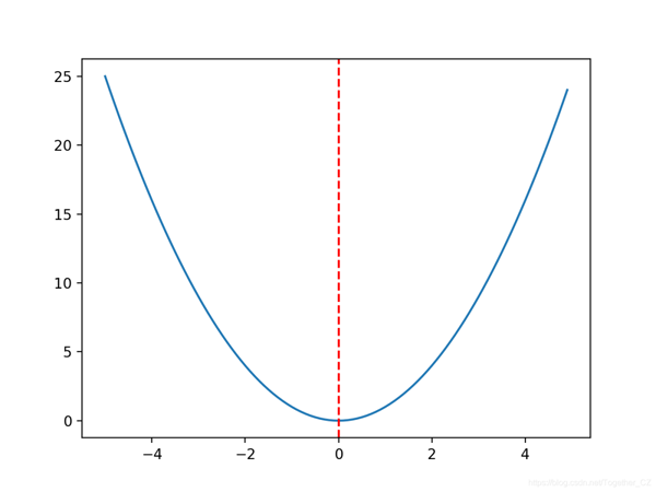
在本節中,我們將把爬山優化算法應用于目標函數。首先,讓我們定義目標函數。我們將使用一個簡單的一維x ^ 2目標函數,其邊界為[-5,5]。下面的示例定義了函數,然后為輸入值的網格創建了函數響應面的折線圖,并用紅線標記了f(0.0)= 0.0處的最佳值。
- # convex unimodal optimization function
- from numpy import arange
- from matplotlib import pyplot
- # objective function
- def objective(x):
- return x[0]**2.0
- # define range for input
- r_min, r_max = -5.0, 5.0
- # sample input range uniformly at 0.1 increments
- inputs = arange(r_min, r_max, 0.1)
- # compute targets
- results = [objective([x]) for x in inputs]
- # create a line plot of input vs result
- pyplot.plot(inputs, results)
- # define optimal input value
- x_optima = 0.0
- # draw a vertical line at the optimal input
- pyplot.axvline(x=x_optima, ls='--', color='red')
- # show the plot
- pyplot.show()
運行示例將創建目標函數的折線圖,并清晰地標記函數的最優值。
接下來,我們可以將爬山算法應用于目標函數。首先,我們將播種偽隨機數生成器。通常這不是必需的,但是在這種情況下,我想確保每次運行算法時都得到相同的結果(相同的隨機數序列),以便以后可以繪制結果。
- # seed the pseudorandom number generator
- seed(5)
接下來,我們可以定義搜索的配置。在這種情況下,我們將搜索算法的1,000次迭代,并使用0.1的步長。假設我們使用的是高斯函數來生成步長,這意味著大約99%的所有步長將位于給定點(0.1 * 3)的距離內,例如 三個標準差。
- n_iterations = 1000
- # define the maximum step size
- step_size = 0.1
接下來,我們可以執行搜索并報告結果。
- # perform the hill climbing search
- best, score = hillclimbing(objective, bounds, n_iterations, step_size)
- print('Done!')
- print('f(%s) = %f' % (best, score))
結合在一起,下面列出了完整的示例。
- # hill climbing search of a one-dimensional objective function
- from numpy import asarray
- from numpy.random import randn
- from numpy.random import rand
- from numpy.random import seed
- # objective function
- def objective(x):
- return x[0]**2.0
- # hill climbing local search algorithm
- def hillclimbing(objective, bounds, n_iterations, step_size):
- # generate an initial point
- solution = bounds[:, 0] + rand(len(bounds)) * (bounds[:, 1] - bounds[:, 0])
- # evaluate the initial point
- solution_eval = objective(solution)
- # run the hill climb
- for i in range(n_iterations):
- # take a step
- candidate = solution + randn(len(bounds)) * step_size
- # evaluate candidate point
- candidte_eval = objective(candidate)
- # check if we should keep the new point
- if candidte_eval <= solution_eval:
- # store the new point
- solution, solution_eval = candidate, candidte_eval
- # report progress
- print('>%d f(%s) = %.5f' % (i, solution, solution_eval))
- return [solution, solution_eval]
- # seed the pseudorandom number generator
- seed(5)
- # define range for input
- bounds = asarray([[-5.0, 5.0]])
- # define the total iterations
- n_iterations = 1000
- # define the maximum step size
- step_size = 0.1
- # perform the hill climbing search
- best, score = hillclimbing(objective, bounds, n_iterations, step_size)
- print('Done!')
- print('f(%s) = %f' % (best, score))
運行該示例將報告搜索進度,包括每次檢測到改進時的迭代次數,該函數的輸入以及來自目標函數的響應。搜索結束時,找到最佳解決方案,并報告其評估結果。在這種情況下,我們可以看到在算法的1,000次迭代中有36處改進,并且該解決方案非常接近于0.0的最佳輸入,其計算結果為f(0.0)= 0.0。
- >1 f([-2.74290923]) = 7.52355
- >3 f([-2.65873147]) = 7.06885
- >4 f([-2.52197291]) = 6.36035
- >5 f([-2.46450214]) = 6.07377
- >7 f([-2.44740961]) = 5.98981
- >9 f([-2.28364676]) = 5.21504
- >12 f([-2.19245939]) = 4.80688
- >14 f([-2.01001538]) = 4.04016
- >15 f([-1.86425287]) = 3.47544
- >22 f([-1.79913002]) = 3.23687
- >24 f([-1.57525573]) = 2.48143
- >25 f([-1.55047719]) = 2.40398
- >26 f([-1.51783757]) = 2.30383
- >27 f([-1.49118756]) = 2.22364
- >28 f([-1.45344116]) = 2.11249
- >30 f([-1.33055275]) = 1.77037
- >32 f([-1.17805016]) = 1.38780
- >33 f([-1.15189314]) = 1.32686
- >36 f([-1.03852644]) = 1.07854
- >37 f([-0.99135322]) = 0.98278
- >38 f([-0.79448984]) = 0.63121
- >39 f([-0.69837955]) = 0.48773
- >42 f([-0.69317313]) = 0.48049
- >46 f([-0.61801423]) = 0.38194
- >48 f([-0.48799625]) = 0.23814
- >50 f([-0.22149135]) = 0.04906
- >54 f([-0.20017144]) = 0.04007
- >57 f([-0.15994446]) = 0.02558
- >60 f([-0.15492485]) = 0.02400
- >61 f([-0.03572481]) = 0.00128
- >64 f([-0.03051261]) = 0.00093
- >66 f([-0.0074283]) = 0.00006
- >78 f([-0.00202357]) = 0.00000
- >119 f([0.00128373]) = 0.00000
- >120 f([-0.00040911]) = 0.00000
- >314 f([-0.00017051]) = 0.00000
- Done!
- f([-0.00017051]) = 0.000000
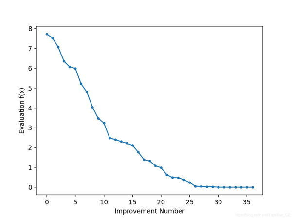
以線圖的形式查看搜索的進度可能很有趣,該線圖顯示了每次改進后最佳解決方案的評估變化。每當有改進時,我們就可以更新hillclimbing()來跟蹤目標函數的評估,并返回此分數列表。
- # hill climbing local search algorithm
- def hillclimbing(objective, bounds, n_iterations, step_size):
- # generate an initial point
- solution = bounds[:, 0] + rand(len(bounds)) * (bounds[:, 1] - bounds[:, 0])
- # evaluate the initial point
- solution_eval = objective(solution)
- # run the hill climb
- scores = list()
- scores.append(solution_eval)
- for i in range(n_iterations):
- # take a step
- candidate = solution + randn(len(bounds)) * step_size
- # evaluate candidate point
- candidte_eval = objective(candidate)
- # check if we should keep the new point
- if candidte_eval <= solution_eval:
- # store the new point
- solution, solution_eval = candidate, candidte_eval
- # keep track of scores
- scores.append(solution_eval)
- # report progress
- print('>%d f(%s) = %.5f' % (i, solution, solution_eval))
- return [solution, solution_eval, scores]
然后,我們可以創建這些分數的折線圖,以查看搜索過程中發現的每個改進的目標函數的相對變化。
- # line plot of best scores
- pyplot.plot(scores, '.-')
- pyplot.xlabel('Improvement Number')
- pyplot.ylabel('Evaluation f(x)')
- pyplot.show()
結合在一起,下面列出了執行搜索并繪制搜索過程中改進解決方案的目標函數得分的完整示例。
- # hill climbing search of a one-dimensional objective function
- from numpy import asarray
- from numpy.random import randn
- from numpy.random import rand
- from numpy.random import seed
- from matplotlib import pyplot
- # objective function
- def objective(x):
- return x[0]**2.0
- # hill climbing local search algorithm
- def hillclimbing(objective, bounds, n_iterations, step_size):
- # generate an initial point
- solution = bounds[:, 0] + rand(len(bounds)) * (bounds[:, 1] - bounds[:, 0])
- # evaluate the initial point
- solution_eval = objective(solution)
- # run the hill climb
- scores = list()
- scores.append(solution_eval)
- for i in range(n_iterations):
- # take a step
- candidate = solution + randn(len(bounds)) * step_size
- # evaluate candidate point
- candidte_eval = objective(candidate)
- # check if we should keep the new point
- if candidte_eval <= solution_eval:
- # store the new point
- solution, solution_eval = candidate, candidte_eval
- # keep track of scores
- scores.append(solution_eval)
- # report progress
- print('>%d f(%s) = %.5f' % (i, solution, solution_eval))
- return [solution, solution_eval, scores]
- # seed the pseudorandom number generator
- seed(5)
- # define range for input
- bounds = asarray([[-5.0, 5.0]])
- # define the total iterations
- n_iterations = 1000
- # define the maximum step size
- step_size = 0.1
- # perform the hill climbing search
- best, score, scores = hillclimbing(objective, bounds, n_iterations, step_size)
- print('Done!')
- print('f(%s) = %f' % (best, score))
- # line plot of best scores
- pyplot.plot(scores, '.-')
- pyplot.xlabel('Improvement Number')
- pyplot.ylabel('Evaluation f(x)')
- pyplot.show()
運行示例將執行搜索,并像以前一樣報告結果。創建一個線形圖,顯示在爬山搜索期間每個改進的目標函數評估。在搜索過程中,我們可以看到目標函數評估發生了約36個變化,隨著算法收斂到最優值,初始變化較大,而在搜索結束時變化很小,難以察覺。
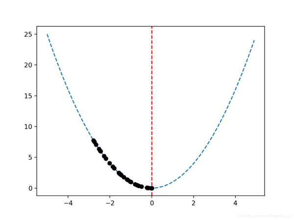
鑒于目標函數是一維的,因此可以像上面那樣直接繪制響應面。通過將在搜索過程中找到的最佳候選解決方案繪制為響應面中的點,來回顧搜索的進度可能會很有趣。我們期望沿著響應面到達最優點的一系列點。這可以通過首先更新hillclimbing()函數以跟蹤每個最佳候選解決方案在搜索過程中的位置來實現,然后返回最佳解決方案列表來實現。
- # hill climbing local search algorithm
- def hillclimbing(objective, bounds, n_iterations, step_size):
- # generate an initial point
- solution = bounds[:, 0] + rand(len(bounds)) * (bounds[:, 1] - bounds[:, 0])
- # evaluate the initial point
- solution_eval = objective(solution)
- # run the hill climb
- solutions = list()
- solutions.append(solution)
- for i in range(n_iterations):
- # take a step
- candidate = solution + randn(len(bounds)) * step_size
- # evaluate candidate point
- candidte_eval = objective(candidate)
- # check if we should keep the new point
- if candidte_eval <= solution_eval:
- # store the new point
- solution, solution_eval = candidate, candidte_eval
- # keep track of solutions
- solutions.append(solution)
- # report progress
- print('>%d f(%s) = %.5f' % (i, solution, solution_eval))
- return [solution, solution_eval, solutions]
然后,我們可以創建目標函數響應面的圖,并像以前那樣標記最優值。
- # sample input range uniformly at 0.1 increments
- inputs = arange(bounds[0,0], bounds[0,1], 0.1)
- # create a line plot of input vs result
- pyplot.plot(inputs, [objective([x]) for x in inputs], '--')
- # draw a vertical line at the optimal input
- pyplot.axvline(x=[0.0], ls='--', color='red')
最后,我們可以將搜索找到的候選解的序列繪制成黑點。
- # plot the sample as black circles
- pyplot.plot(solutions, [objective(x) for x in solutions], 'o', color='black')
結合在一起,下面列出了在目標函數的響應面上繪制改進解序列的完整示例。
- # hill climbing search of a one-dimensional objective function
- from numpy import asarray
- from numpy import arange
- from numpy.random import randn
- from numpy.random import rand
- from numpy.random import seed
- from matplotlib import pyplot
- # objective function
- def objective(x):
- return x[0]**2.0
- # hill climbing local search algorithm
- def hillclimbing(objective, bounds, n_iterations, step_size):
- # generate an initial point
- solution = bounds[:, 0] + rand(len(bounds)) * (bounds[:, 1] - bounds[:, 0])
- # evaluate the initial point
- solution_eval = objective(solution)
- # run the hill climb
- solutions = list()
- solutions.append(solution)
- for i in range(n_iterations):
- # take a step
- candidate = solution + randn(len(bounds)) * step_size
- # evaluate candidate point
- candidte_eval = objective(candidate)
- # check if we should keep the new point
- if candidte_eval <= solution_eval:
- # store the new point
- solution, solution_eval = candidate, candidte_eval
- # keep track of solutions
- solutions.append(solution)
- # report progress
- print('>%d f(%s) = %.5f' % (i, solution, solution_eval))
- return [solution, solution_eval, solutions]
- # seed the pseudorandom number generator
- seed(5)
- # define range for input
- bounds = asarray([[-5.0, 5.0]])
- # define the total iterations
- n_iterations = 1000
- # define the maximum step size
- step_size = 0.1
- # perform the hill climbing search
- best, score, solutions = hillclimbing(objective, bounds, n_iterations, step_size)
- print('Done!')
- print('f(%s) = %f' % (best, score))
- # sample input range uniformly at 0.1 increments
- inputs = arange(bounds[0,0], bounds[0,1], 0.1)
- # create a line plot of input vs result
- pyplot.plot(inputs, [objective([x]) for x in inputs], '--')
- # draw a vertical line at the optimal input
- pyplot.axvline(x=[0.0], ls='--', color='red')
- # plot the sample as black circles
- pyplot.plot(solutions, [objective(x) for x in solutions], 'o', color='black')
- pyplot.show()
運行示例將執行爬山搜索,并像以前一樣報告結果。像以前一樣創建一個響應面圖,顯示函數的熟悉的碗形,并用垂直的紅線標記函數的最佳狀態。在搜索過程中找到的最佳解決方案的順序顯示為黑點,沿著碗形延伸到最佳狀態。