聲音分類是音頻深度學(xué)習(xí)中應(yīng)用最廣泛的方法之一。它包括學(xué)習(xí)對(duì)聲音進(jìn)行分類并預(yù)測(cè)聲音的類別。這類問(wèn)題可以應(yīng)用到許多實(shí)際場(chǎng)景中，例如，對(duì)音樂(lè)片段進(jìn)行分類以識(shí)別音樂(lè)類型，或通過(guò)一組揚(yáng)聲器對(duì)短話語(yǔ)進(jìn)行分類以根據(jù)聲音識(shí)別說(shuō)話人。

[[388733]]

在本文中，我們將介紹一個(gè)簡(jiǎn)單的演示應(yīng)用程序，以便理解用于解決此類音頻分類問(wèn)題的方法。我的目標(biāo)不僅僅是理解事物是如何運(yùn)作的，還有它為什么會(huì)這樣運(yùn)作。

音頻分類

就像使用MNIST數(shù)據(jù)集對(duì)手寫數(shù)字進(jìn)行分類被認(rèn)為是計(jì)算機(jī)視覺(jué)的“Hello World”類型的問(wèn)題一樣，我們可以將此應(yīng)用視為音頻深度學(xué)習(xí)的入門問(wèn)題。

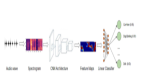
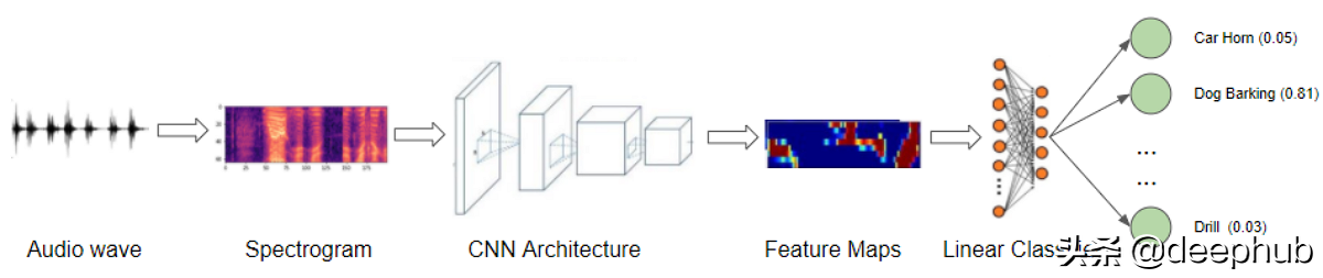
我們將從聲音文件開(kāi)始，將它們轉(zhuǎn)換為聲譜圖，將它們輸入到CNN加線性分類器模型中，并產(chǎn)生關(guān)于聲音所屬類別的預(yù)測(cè)。

有許多合適的數(shù)據(jù)集可以用于不同類型的聲音。這些數(shù)據(jù)集包含大量音頻樣本，以及每個(gè)樣本的類標(biāo)簽，根據(jù)你試圖解決的問(wèn)題來(lái)識(shí)別聲音的類型。

這些類標(biāo)簽通常可以從音頻樣本文件名的某些部分或文件所在的子文件夾名中獲得。另外，類標(biāo)簽在單獨(dú)的元數(shù)據(jù)文件中指定，通常為TXT、JSON或CSV格式。

演示-對(duì)普通城市聲音進(jìn)行分類

對(duì)于我們的演示，我們將使用Urban Sound 8K數(shù)據(jù)集，該數(shù)據(jù)集包含從日常城市生活中錄制的普通聲音的語(yǔ)料庫(kù)。這些聲音來(lái)自于10個(gè)分類，如工程噪音、狗叫聲和汽笛聲。每個(gè)聲音樣本都標(biāo)有它所屬的類。

下載數(shù)據(jù)集后，我們看到它由兩部分組成:

“Audio”文件夾中的音頻文件:它有10個(gè)子文件夾，命名為“fold1”到“fold10”。每個(gè)子文件夾包含許多。wav的音頻樣本。例如“fold1/103074 - 7 - 1 - 0. - wav”

“Metadata”文件夾中的元數(shù)據(jù):它有一個(gè)文件“UrbanSound8K”。它包含關(guān)于數(shù)據(jù)集中每個(gè)音頻樣本的信息，如文件名、類標(biāo)簽、“fold”子文件夾位置等。類標(biāo)簽是10個(gè)類中的每個(gè)類從0到9的數(shù)字類ID。如。數(shù)字0表示空調(diào)，1表示汽車?yán)龋源祟愅啤?/p>

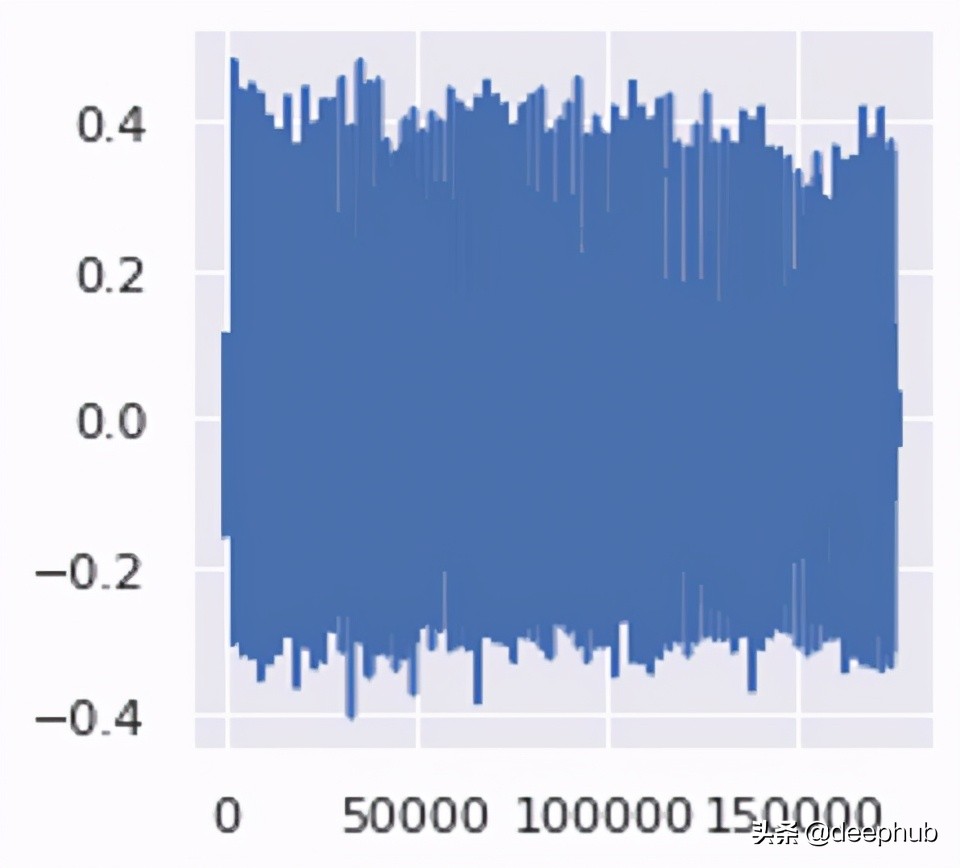
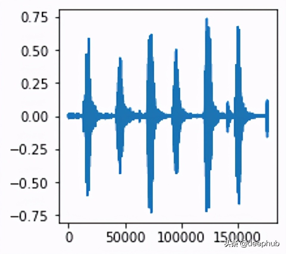
一般音頻的長(zhǎng)度約為4秒。下面是其中一個(gè)例子:

數(shù)據(jù)集創(chuàng)建者的建議是使用10折的交叉驗(yàn)證，以便計(jì)算指標(biāo)并評(píng)估模型的性能。 但是，由于本文的目標(biāo)主要是作為音頻深度學(xué)習(xí)示例的演示，而不是獲得最佳指標(biāo)，因此，我們將忽略分折并將所有樣本簡(jiǎn)單地視為一個(gè)大型數(shù)據(jù)集。

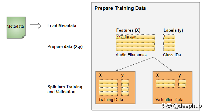
準(zhǔn)備訓(xùn)練數(shù)據(jù)

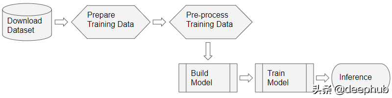
對(duì)于大多數(shù)深度學(xué)習(xí)問(wèn)題，我們將遵循以下步驟:

這個(gè)數(shù)據(jù)集的數(shù)據(jù)整理很簡(jiǎn)單:

特性(X)是音頻文件路徑

目標(biāo)標(biāo)簽(y)是類名

由于數(shù)據(jù)集已經(jīng)有一個(gè)包含此信息的元數(shù)據(jù)文件，所以我們可以直接使用它。元數(shù)據(jù)包含關(guān)于每個(gè)音頻文件的信息。

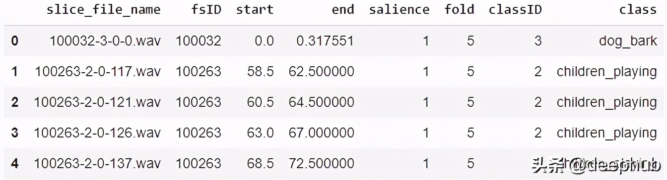
由于它是一個(gè)CSV文件，我們可以使用Pandas來(lái)讀取它。我們可以從元數(shù)據(jù)中準(zhǔn)備特性和標(biāo)簽數(shù)據(jù)。

# ----------------------------  
# Prepare training data from Metadata file  
# ----------------------------  
import pandas as pd  
from pathlib import Path  
 
download_path = Path.cwd()/'UrbanSound8K'  
 
# Read metadata file  
metadata_file = download_path/'metadata'/'UrbanSound8K.csv'  
df = pd.read_csv(metadata_file)  
df.head()  
 
# Construct file path by concatenating fold and file name  
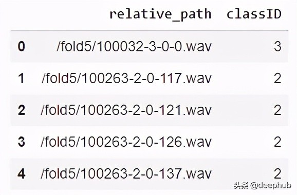
df['relative_path'] = '/fold' + df['fold'].astype(str) + '/' + df['slice_file_name'].astype(str)  
 
# Take relevant columns  
df = df[['relative_path', 'classID']]  
df.head() 

我們訓(xùn)練的需要的信息如下：

當(dāng)元數(shù)據(jù)不可用時(shí)，掃描音頻文件目錄

有了元數(shù)據(jù)文件，事情就簡(jiǎn)單多了。我們?nèi)绾螢椴话獢?shù)據(jù)文件的數(shù)據(jù)集準(zhǔn)備數(shù)據(jù)呢?

許多數(shù)據(jù)集僅包含安排在文件夾結(jié)構(gòu)中的音頻文件，類標(biāo)簽可以通過(guò)目錄進(jìn)行派生。為了以這種格式準(zhǔn)備我們的培訓(xùn)數(shù)據(jù)，我們將做以下工作:

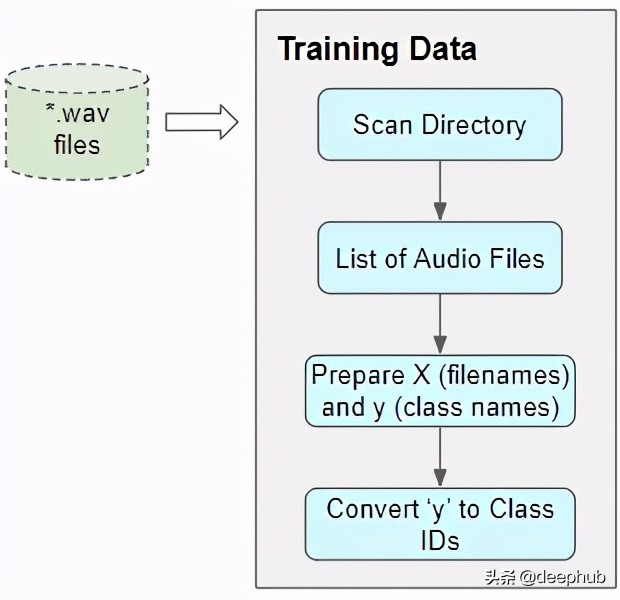
掃描該目錄并生成所有音頻文件路徑的列表。

從每個(gè)文件名或父子文件夾的名稱中提取類標(biāo)簽

將每個(gè)類名從文本映射到一個(gè)數(shù)字類ID

不管有沒(méi)有元數(shù)據(jù)，結(jié)果都是一樣的——由音頻文件名列表組成的特性和由類id組成的目標(biāo)標(biāo)簽。

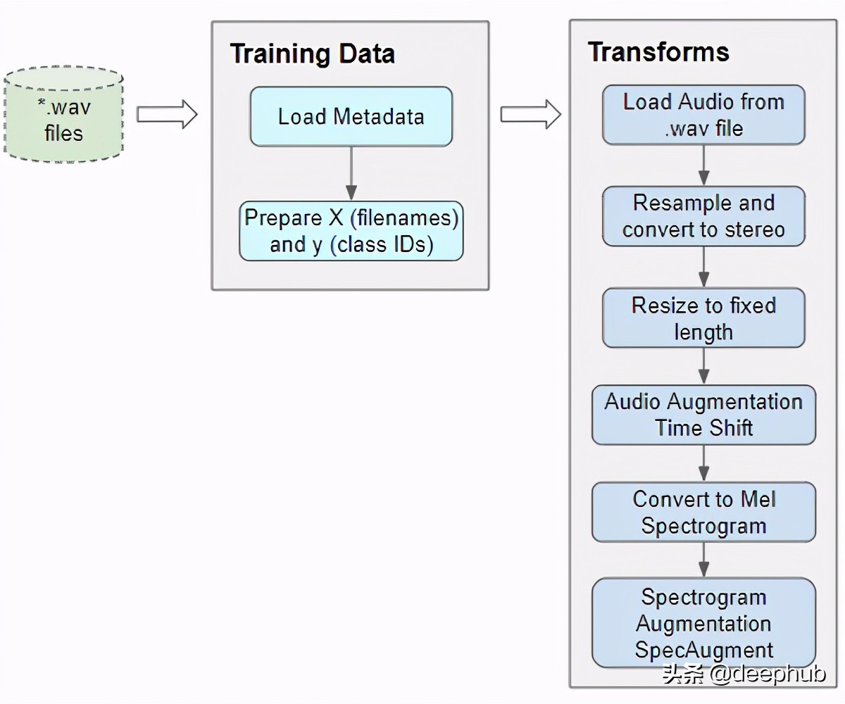
音頻預(yù)處理:定義變換

這種帶有音頻文件路徑的訓(xùn)練數(shù)據(jù)不能直接輸入到模型中。我們必須從文件中加載音頻數(shù)據(jù)并對(duì)其進(jìn)行處理，使其符合模型所期望的格式。

當(dāng)我們讀取并加載音頻文件時(shí)，所有音頻預(yù)處理將在運(yùn)行時(shí)動(dòng)態(tài)完成。這種方法也類似于我們將要處理的圖像文件。由于音頻數(shù)據(jù)(或圖像數(shù)據(jù))可能非常大且占用大量?jī)?nèi)存，因此我們不希望提前一次將整個(gè)數(shù)據(jù)集全部讀取到內(nèi)存中。因此，我們?cè)谟?xùn)練數(shù)據(jù)中僅保留音頻文件名(或圖像文件名)。。

然后在運(yùn)行時(shí)，當(dāng)我們一次訓(xùn)練一批數(shù)據(jù)時(shí)，我們將加載該批次的音頻數(shù)據(jù)，并通過(guò)對(duì)音頻進(jìn)行一系列轉(zhuǎn)換來(lái)對(duì)其進(jìn)行處理。這樣，我們一次只將一批音頻數(shù)據(jù)保存在內(nèi)存中。

對(duì)于圖像數(shù)據(jù)，我們可能會(huì)有一個(gè)轉(zhuǎn)換管道，在該轉(zhuǎn)換過(guò)程中，我們首先將圖像文件讀取為像素并將其加載。然后，我們可以應(yīng)用一些圖像處理步驟來(lái)調(diào)整數(shù)據(jù)的形狀和大小，將其裁剪為固定大小，然后將其從RGB轉(zhuǎn)換為灰度(如果需要)。我們可能還會(huì)應(yīng)用一些圖像增強(qiáng)步驟，例如旋轉(zhuǎn)，翻轉(zhuǎn)等。

音頻數(shù)據(jù)的處理非常相似。現(xiàn)在我們只定義函數(shù)，當(dāng)我們?cè)谟?xùn)練期間向模型提供數(shù)據(jù)時(shí)，它們將在稍后運(yùn)行。

讀取文件中的音頻

我們需要做的第一件事是以“ .wav”格式讀取和加載音頻文件。 由于我們?cè)诖耸纠惺褂玫氖荘ytorch，因此下面的實(shí)現(xiàn)使用torchaudio進(jìn)行音頻處理，但是librosa也可以正常工作。

import math, random  
import torch  
import torchaudio  
from torchaudio import transforms  
from IPython.display import Audio  
 
class AudioUtil():  
# ----------------------------  
# Load an audio file. Return the signal as a tensor and the sample rate  
# ----------------------------  
@staticmethod  
def open(audio_file):  
sig, sr = torchaudio.load(audio_file)  
return (sig, sr) 

轉(zhuǎn)換成立體聲

一些聲音文件是單聲道(即1個(gè)音頻通道)，而大多數(shù)則是立體聲(即2個(gè)音頻通道)。 由于我們的模型期望所有項(xiàng)目都具有相同的尺寸，因此我們將第一個(gè)通道復(fù)制到第二個(gè)通道，從而將單聲道文件轉(zhuǎn)換為立體聲。

# ----------------------------  
# Convert the given audio to the desired number of channels  
# ----------------------------  
@staticmethod  
def rechannel(aud, new_channel):  
sig, sr = aud  
 
if (sig.shape[0] == new_channel):  
# Nothing to do  
return aud  
 
if (new_channel == 1):  
# Convert from stereo to mono by selecting only the first channel  
resig = sig[:1, :]  
else:  
# Convert from mono to stereo by duplicating the first channel  
resig = torch.cat([sig, sig])  
 
return ((resig, sr)) 

標(biāo)準(zhǔn)化采樣率

一些聲音文件以48000Hz的采樣率采樣，而大多數(shù)聲音文件以44100Hz的采樣率采樣。 這意味著對(duì)于某些聲音文件，1秒音頻的數(shù)組大小為48000，而對(duì)于其他聲音文件，其數(shù)組大小為44100。 ，我們必須將所有音頻標(biāo)準(zhǔn)化并將其轉(zhuǎn)換為相同的采樣率，以使所有陣列具有相同的尺寸。

# ----------------------------  
# Since Resample applies to a single channel, we resample one channel at a time  
# ----------------------------  
@staticmethod  
def resample(aud, newsr):  
sig, sr = aud  
 
if (sr == newsr):  
# Nothing to do  
return aud  
 
num_channels = sig.shape[0]  
# Resample first channel  
resig = torchaudio.transforms.Resample(sr, newsr)(sig[:1,:])  
if (num_channels > 1):  
# Resample the second channel and merge both channels  
retwo = torchaudio.transforms.Resample(sr, newsr)(sig[1:,:])  
resig = torch.cat([resig, retwo])  
 
return ((resig, newsr)) 

調(diào)整為相同長(zhǎng)度

然后，我們將所有音頻樣本的大小調(diào)整為具有相同的長(zhǎng)度，方法是通過(guò)使用靜默填充或通過(guò)截?cái)嗥溟L(zhǎng)度來(lái)延長(zhǎng)其持續(xù)時(shí)間。 我們將該方法添加到AudioUtil類中。

# ----------------------------  
# Pad (or truncate) the signal to a fixed length 'max_ms' in milliseconds  
# ----------------------------  
@staticmethod  
def pad_trunc(aud, max_ms):  
sig, sr = aud  
num_rows, sig_len = sig.shape  
max_len = sr//1000 * max_ms  
 
if (sig_len > max_len):  
# Truncate the signal to the given length  
sig = sig[:,:max_len]  
 
elif (sig_len < max_len):  
# Length of padding to add at the beginning and end of the signal  
pad_begin_len = random.randint(0, max_len - sig_len)  
pad_end_len = max_len - sig_len - pad_begin_len  
 
# Pad with 0s  
pad_begin = torch.zeros((num_rows, pad_begin_len))  
pad_end = torch.zeros((num_rows, pad_end_len))  
 
sig = torch.cat((pad_begin, sig, pad_end), 1)  
 
return (sig, sr) 

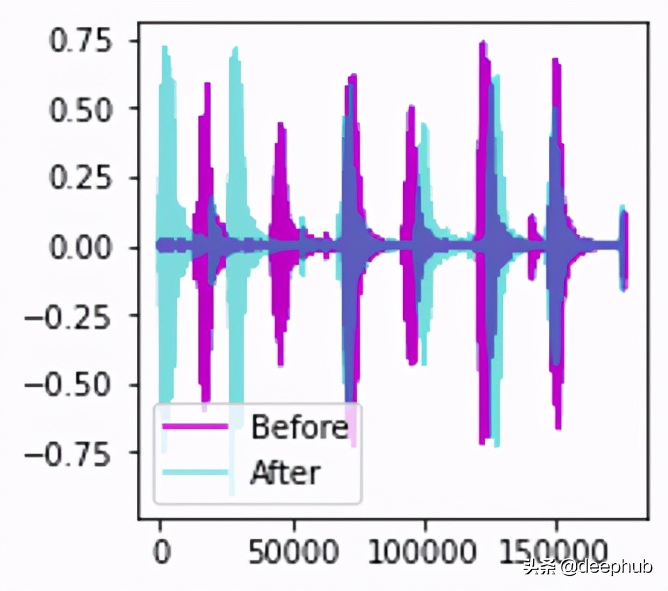
數(shù)據(jù)擴(kuò)充增廣：時(shí)移

接下來(lái)，我們可以通過(guò)應(yīng)用時(shí)間偏移將音頻向左或向右移動(dòng)隨機(jī)量來(lái)對(duì)原始音頻信號(hào)進(jìn)行數(shù)據(jù)增廣。 在本文中，我將詳細(xì)介紹此技術(shù)和其他數(shù)據(jù)增廣技術(shù)。

# ----------------------------  
# Shifts the signal to the left or right by some percent. Values at the end  
# are 'wrapped around' to the start of the transformed signal.  
# ----------------------------  
@staticmethod  
def time_shift(aud, shift_limit):  
sig,sr = aud  
_, sig_len = sig.shape  
shift_amt = int(random.random() * shift_limit * sig_len)  
return (sig.roll(shift_amt), sr) 

梅爾譜圖

我們將增廣后的音頻轉(zhuǎn)換為梅爾頻譜圖。 它們捕獲了音頻的基本特征，并且通常是將音頻數(shù)據(jù)輸入到深度學(xué)習(xí)模型中的最合適方法。

# ----------------------------  
# Generate a Spectrogram  
# ----------------------------  
@staticmethod  
def spectro_gram(aud, n_mels=64, n_fft=1024, hop_len=None):  
sig,sr = aud  
top_db = 80  
 
# spec has shape [channel, n_mels, time], where channel is mono, stereo etc  
spec = transforms.MelSpectrogram(sr, n_fft=n_fft, hop_length=hop_len, n_mels=n_mels)(sig)  
 
# Convert to decibels  
spec = transforms.AmplitudeToDB(top_db=top_db)(spec)  
return (spec) 

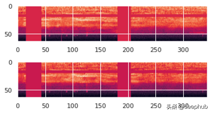
數(shù)據(jù)擴(kuò)充：時(shí)間和頻率屏蔽

現(xiàn)在我們可以進(jìn)行另一輪擴(kuò)充，這次是在Mel頻譜圖上，而不是在原始音頻上。 我們將使用一種稱為SpecAugment的技術(shù)，該技術(shù)使用以下兩種方法：

頻率屏蔽-通過(guò)在頻譜圖上添加水平條來(lái)隨機(jī)屏蔽一系列連續(xù)頻率。

時(shí)間掩碼-與頻率掩碼類似，不同之處在于，我們使用豎線從頻譜圖中隨機(jī)地遮擋了時(shí)間范圍。

# ----------------------------  
# Augment the Spectrogram by masking out some sections of it in both the frequency  
# dimension (ie. horizontal bars) and the time dimension (vertical bars) to prevent  
# overfitting and to help the model generalise better. The masked sections are  
# replaced with the mean value.  
# ----------------------------  
@staticmethod  
def spectro_augment(spec, max_mask_pct=0.1, n_freq_masks=1, n_time_masks=1):  
_, n_mels, n_steps = spec.shape  
mask_value = spec.mean()  
aug_spec = spec  
 
freq_mask_param = max_mask_pct * n_mels  
for _ in range(n_freq_masks):  
aug_spec = transforms.FrequencyMasking(freq_mask_param)(aug_spec, mask_value)  
 
time_mask_param = max_mask_pct * n_steps  
for _ in range(n_time_masks):  
aug_spec = transforms.TimeMasking(time_mask_param)(aug_spec, mask_value)  
 
return aug_spec 

自定義數(shù)據(jù)加載器

現(xiàn)在，我們已經(jīng)定義了所有預(yù)處理轉(zhuǎn)換函數(shù)，我們將定義一個(gè)自定義的Pytorch Dataset對(duì)象。

要將數(shù)據(jù)提供給使用Pytorch的模型，我們需要兩個(gè)對(duì)象：

一個(gè)自定義Dataset對(duì)象，該對(duì)象使用所有音頻轉(zhuǎn)換來(lái)預(yù)處理音頻文件并一次準(zhǔn)備一個(gè)數(shù)據(jù)項(xiàng)。

內(nèi)置的DataLoader對(duì)象，該對(duì)象使用Dataset對(duì)象來(lái)獲取單個(gè)數(shù)據(jù)項(xiàng)并將其打包為一批數(shù)據(jù)。

from torch.utils.data import DataLoader, Dataset, random_split  
import torchaudio  
 
# ----------------------------  
# Sound Dataset  
# ----------------------------  
class SoundDS(Dataset):  
def __init__(self, df, data_path):  
self.df = df  
self.data_path = str(data_path)  
self.duration = 4000  
self.sr = 44100  
self.channel = 2  
self.shift_pct = 0.4  
 
# ----------------------------  
# Number of items in dataset  
# ----------------------------  
def __len__(self):  
return len(self.df)  
 
# ----------------------------  
# Get i'th item in dataset  
# ----------------------------  
def __getitem__(self, idx):  
# Absolute file path of the audio file - concatenate the audio directory with  
# the relative path  
audio_file = self.data_path + self.df.loc[idx, 'relative_path']  
# Get the Class ID  
class_id = self.df.loc[idx, 'classID']  
 
aud = AudioUtil.open(audio_file)  
# Some sounds have a higher sample rate, or fewer channels compared to the  
# majority. So make all sounds have the same number of channels and same  
# sample rate. Unless the sample rate is the same, the pad_trunc will still  
# result in arrays of different lengths, even though the sound duration is  
# the same.  
reaud = AudioUtil.resample(aud, self.sr)  
rechan = AudioUtil.rechannel(reaud, self.channel)  
 
dur_aud = AudioUtil.pad_trunc(rechan, self.duration)  
shift_aud = AudioUtil.time_shift(dur_aud, self.shift_pct)  
sgram = AudioUtil.spectro_gram(shift_aud, n_mels=64, n_fft=1024, hop_len=None)  
aug_sgram = AudioUtil.spectro_augment(sgram, max_mask_pct=0.1, n_freq_masks=2, n_time_masks=2)  
 
return aug_sgram, class_id 

使用數(shù)據(jù)加載器準(zhǔn)備一批數(shù)據(jù)

現(xiàn)在已經(jīng)定義了我們需要將數(shù)據(jù)輸入到模型中的所有函數(shù)。

我們使用自定義數(shù)據(jù)集從Pandas中加載特征和標(biāo)簽，然后以80:20的比例將數(shù)據(jù)隨機(jī)分為訓(xùn)練和驗(yàn)證集。 然后，我們使用它們來(lái)創(chuàng)建我們的訓(xùn)練和驗(yàn)證數(shù)據(jù)加載器。

from torch.utils.data import random_split  
 
myds = SoundDS(df, data_path)  
 
# Random split of 80:20 between training and validation  
num_items = len(myds)  
num_train = round(num_items * 0.8)  
num_val = num_items - num_train  
train_ds, val_ds = random_split(myds, [num_train, num_val])  
 
# Create training and validation data loaders  
train_dl = torch.utils.data.DataLoader(train_ds, batch_size=16, shuffle=True)  
val_dl = torch.utils.data.DataLoader(val_ds, batch_size=16, shuffle=False) 

當(dāng)我們開(kāi)始訓(xùn)練時(shí)，將隨機(jī)獲取一批包含音頻文件名列表的輸入，并在每個(gè)音頻文件上運(yùn)行預(yù)處理音頻轉(zhuǎn)換。 它還將獲取一批包含類ID的相應(yīng)目標(biāo)Label。 因此，它將一次輸出一批訓(xùn)練數(shù)據(jù)，這些數(shù)據(jù)可以直接作為輸入提供給我們的深度學(xué)習(xí)模型。

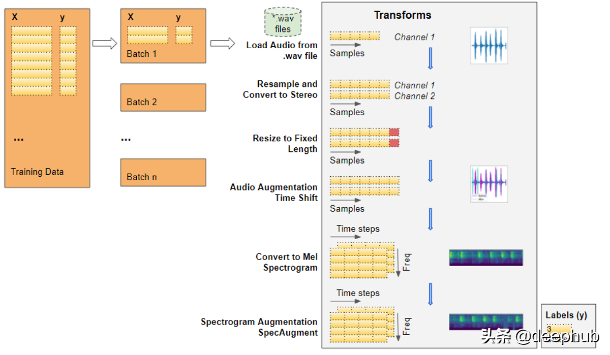
讓我們從音頻文件開(kāi)始，逐步完成數(shù)據(jù)轉(zhuǎn)換的各個(gè)步驟：

文件中的音頻被加載到Numpy的數(shù)組中(numchannels，numsamples)。大部分音頻以44.1kHz采樣，持續(xù)時(shí)間約為4秒，從而產(chǎn)生44,100 * 4 = 176,400個(gè)采樣。如果音頻具有1個(gè)通道，則陣列的形狀將為(1、176,400)。同樣，具有2個(gè)通道的4秒鐘持續(xù)時(shí)間且以48kHz采樣的音頻將具有192,000個(gè)采樣，形狀為(2，192,000)。

每種音頻的通道和采樣率不同，因此接下來(lái)的兩次轉(zhuǎn)換會(huì)將音頻重新采樣為標(biāo)準(zhǔn)的44.1kHz和標(biāo)準(zhǔn)的2個(gè)通道。

某些音頻片段可能大于或小于4秒，因此我們還將音頻持續(xù)時(shí)間標(biāo)準(zhǔn)化為固定的4秒長(zhǎng)度。現(xiàn)在，所有項(xiàng)目的數(shù)組都具有相同的形狀(2，176,400)

時(shí)移數(shù)據(jù)擴(kuò)充功能會(huì)隨機(jī)將每個(gè)音頻樣本向前或向后移動(dòng)。形狀不變。

擴(kuò)充后的音頻將轉(zhuǎn)換為梅爾頻譜圖，其形狀為(numchannels，Mel freqbands，time_steps)=(2，64，344)

SpecAugment數(shù)據(jù)擴(kuò)充功能將時(shí)間和頻率掩碼隨機(jī)應(yīng)用于梅爾頻譜圖。形狀不變。

最后我們每批得到了兩個(gè)張量，一個(gè)用于包含梅爾頻譜圖的X特征數(shù)據(jù)，另一個(gè)用于包含數(shù)字類ID的y目標(biāo)標(biāo)簽。 從每個(gè)訓(xùn)練輪次的訓(xùn)練數(shù)據(jù)中隨機(jī)選擇批次。

每個(gè)批次的形狀為(batchsz，numchannels，Mel freqbands，timesteps)

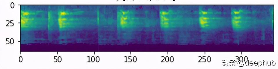
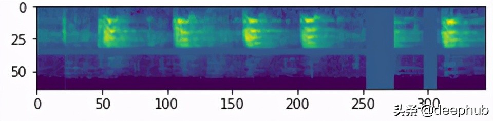
我們可以將批次中的一項(xiàng)可視化。 我們看到帶有垂直和水平條紋的梅爾頻譜圖顯示了頻率和時(shí)間屏蔽數(shù)據(jù)的擴(kuò)充。

建立模型

我們剛剛執(zhí)行的數(shù)據(jù)處理步驟是我們音頻分類問(wèn)題中最獨(dú)特的方面。 從這里開(kāi)始，模型和訓(xùn)練過(guò)程與標(biāo)準(zhǔn)圖像分類問(wèn)題中常用的模型和訓(xùn)練過(guò)程非常相似，并且不特定于音頻深度學(xué)習(xí)。

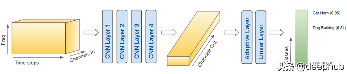
由于我們的數(shù)據(jù)現(xiàn)在由光譜圖圖像組成，因此我們建立了CNN分類架構(gòu)來(lái)對(duì)其進(jìn)行處理。 它具有生成特征圖的四個(gè)卷積塊。 然后將數(shù)據(jù)重新整形為我們需要的格式，以便可以將其輸入到線性分類器層，該層最終輸出針對(duì)10個(gè)分類的預(yù)測(cè)。

模型信息：

色彩圖像以形狀(batchsz，numchannels，Mel freqbands，timesteps)輸入模型。(16，2，64，344)。

每個(gè)CNN層都應(yīng)用其濾鏡以提高圖像深度，即通道數(shù)。 (16、64、4、22)。

將其合并并展平為(16，64)的形狀，然后輸入到“線性”層。

線性層為每個(gè)類別輸出一個(gè)預(yù)測(cè)分?jǐn)?shù)，即(16、10)

import torch.nn.functional as F  
from torch.nn import init  
 
# ----------------------------  
# Audio Classification Model  
# ----------------------------  
class AudioClassifier (nn.Module):  
# ----------------------------  
# Build the model architecture  
# ----------------------------  
def __init__(self):  
super().__init__()  
conv_layers = []  
 
# First Convolution Block with Relu and Batch Norm. Use Kaiming Initialization  
self.conv1 = nn.Conv2d(2, 8, kernel_size=(5, 5), stride=(2, 2), padding=(2, 2))  
self.relu1 = nn.ReLU()  
self.bn1 = nn.BatchNorm2d(8)  
init.kaiming_normal_(self.conv1.weight, a=0.1)  
self.conv1.bias.data.zero_()  
conv_layers += [self.conv1, self.relu1, self.bn1]  
 
# Second Convolution Block  
self.conv2 = nn.Conv2d(8, 16, kernel_size=(3, 3), stride=(2, 2), padding=(1, 1))  
self.relu2 = nn.ReLU()  
self.bn2 = nn.BatchNorm2d(16)  
init.kaiming_normal_(self.conv2.weight, a=0.1)  
self.conv2.bias.data.zero_()  
conv_layers += [self.conv2, self.relu2, self.bn2]  
 
# Second Convolution Block  
self.conv3 = nn.Conv2d(16, 32, kernel_size=(3, 3), stride=(2, 2), padding=(1, 1))  
self.relu3 = nn.ReLU()  
self.bn3 = nn.BatchNorm2d(32)  
init.kaiming_normal_(self.conv3.weight, a=0.1)  
self.conv3.bias.data.zero_()  
conv_layers += [self.conv3, self.relu3, self.bn3]  
 
# Second Convolution Block  
self.conv4 = nn.Conv2d(32, 64, kernel_size=(3, 3), stride=(2, 2), padding=(1, 1))  
self.relu4 = nn.ReLU()  
self.bn4 = nn.BatchNorm2d(64)  
init.kaiming_normal_(self.conv4.weight, a=0.1)  
self.conv4.bias.data.zero_()  
conv_layers += [self.conv4, self.relu4, self.bn4]  
 
# Linear Classifier  
self.ap = nn.AdaptiveAvgPool2d(output_size=1)  
self.lin = nn.Linear(in_features=64, out_features=10)  
 
# Wrap the Convolutional Blocks  
self.conv = nn.Sequential(*conv_layers)  
 
# ----------------------------  
# Forward pass computations  
# ----------------------------  
def forward(self, x):  
# Run the convolutional blocks  
x = self.conv(x)  
 
# Adaptive pool and flatten for input to linear layer  
x = self.ap(x)  
x = x.view(x.shape[0], -1)  
 
# Linear layer  
x = self.lin(x)  
 
# Final output  
return x  
 
# Create the model and put it on the GPU if available  
myModel = AudioClassifier()  
device = torch.device("cuda:0" if torch.cuda.is_available() else "cpu")  
myModel = myModel.to(device)  
# Check that it is on Cuda  
next(myModel.parameters()).device 

訓(xùn)練

現(xiàn)在，我們準(zhǔn)備創(chuàng)建訓(xùn)練循環(huán)來(lái)訓(xùn)練模型。

我們定義了優(yōu)化器，損失函數(shù)和學(xué)習(xí)率的調(diào)度計(jì)劃的函數(shù)，以便隨著訓(xùn)練的進(jìn)行而動(dòng)態(tài)地改變我們的學(xué)習(xí)率，這樣可以使模型收斂的更快。

在每輪訓(xùn)練完成后。 我們跟蹤一個(gè)簡(jiǎn)單的準(zhǔn)確性指標(biāo)，該指標(biāo)衡量正確預(yù)測(cè)的百分比。

# ----------------------------

# Training Loop

# ----------------------------

def training(model, train_dl, num_epochs):

# Loss Function, Optimizer and Scheduler

criterion = nn.CrossEntropyLoss()

optimizer = torch.optim.Adam(model.parameters(),lr=0.001)

scheduler = torch.optim.lr_scheduler.OneCycleLR(optimizer, max_lr=0.001,

steps_per_epoch=int(len(train_dl)),

epochs=num_epochs,

anneal_strategy='linear')

# Repeat for each epoch

for epoch in range(num_epochs):

running_loss = 0.0

correct_prediction = 0

total_prediction = 0

# Repeat for each batch in the training set

for i, data in enumerate(train_dl):

# Get the input features and target labels, and put them on the GPU

inputs, labels = data[0].to(device), data[1].to(device)

# Normalize the inputs

inputs_m, inputs_s = inputs.mean(), inputs.std()

inputs = (inputs - inputs_m) / inputs_s

# Zero the parameter gradients

optimizer.zero_grad()

# forward + backward + optimize

outputs = model(inputs)

loss = criterion(outputs, labels)

loss.backward()

optimizer.step()

scheduler.step()

# Keep stats for Loss and Accuracy

running_loss += loss.item()

# Get the predicted class with the highest score

_, prediction = torch.max(outputs,1)

# Count of predictions that matched the target label

correct_prediction += (prediction == labels).sum().item()

total_prediction += prediction.shape[0]

#if i % 10 == 0: # print every 10 mini-batches

# print('[%d, %5d] loss: %.3f' % (epoch + 1, i + 1, running_loss / 10))

# Print stats at the end of the epoch

num_batches = len(train_dl)

avg_loss = running_loss / num_batches

acc = correct_prediction/total_prediction

print(f'Epoch: {epoch}, Loss: {avg_loss:.2f}, Accuracy: {acc:.2f}')

print('Finished Training')

num_epochs=2 # Just for demo, adjust this higher.

training(myModel, train_dl, num_epochs)

推理

通常，作為訓(xùn)練循環(huán)的一部分，我們還將根據(jù)驗(yàn)證數(shù)據(jù)評(píng)估指標(biāo)。 所以我們會(huì)對(duì)原始數(shù)據(jù)中保留測(cè)試數(shù)據(jù)集(被當(dāng)作是訓(xùn)練時(shí)看不見(jiàn)的數(shù)據(jù))進(jìn)行推理。 出于本演示的目的，我們將為此目的使用驗(yàn)證數(shù)據(jù)。

我們禁用梯度更新并運(yùn)行一個(gè)推理循環(huán)。 與模型一起執(zhí)行前向傳播以獲取預(yù)測(cè)，但是我們不需要反向傳播和優(yōu)化。

# ----------------------------  
# Inference  
# ----------------------------  
def inference (model, val_dl):  
correct_prediction = 0  
total_prediction = 0  
 
# Disable gradient updates  
with torch.no_grad():  
for data in val_dl:  
# Get the input features and target labels, and put them on the GPU  
inputs, labels = data[0].to(device), data[1].to(device)  
 
# Normalize the inputs  
inputs_m, inputs_s = inputs.mean(), inputs.std()  
inputs = (inputs - inputs_m) / inputs_s  
 
# Get predictions  
outputs = model(inputs)  
 
# Get the predicted class with the highest score  
_, prediction = torch.max(outputs,1)  
# Count of predictions that matched the target label  
correct_prediction += (prediction == labels).sum().item()  
total_prediction += prediction.shape[0]  
 
acc = correct_prediction/total_prediction  
print(f'Accuracy: {acc:.2f}, Total items: {total_prediction}')  
 
# Run inference on trained model with the validation set  
inference(myModel, val_dl) 

結(jié)論

現(xiàn)在我們已經(jīng)看到了聲音分類的端到端示例，它是音頻深度學(xué)習(xí)中最基礎(chǔ)的問(wèn)題之一。 這不僅可以用于廣泛的應(yīng)用中，而且我們?cè)诖私榻B的許多概念和技術(shù)都將與更復(fù)雜的音頻問(wèn)題相關(guān)，例如自動(dòng)語(yǔ)音識(shí)別，其中我們從人類語(yǔ)音入手，了解人們?cè)谡f(shuō)什么，以及將其轉(zhuǎn)換為文本。