線性回歸,核技巧和線性核
在這篇文章中,我想展示一個有趣的結果:線性回歸與無正則化的線性核ridge回歸是等價的。
這里實際上涉及到很多概念和技術,所以我們將逐一介紹,最后用它們來解釋這個說法。
首先我們回顧經典的線性回歸。然后我將解釋什么是核函數和線性核函數,最后我們將給出上面表述的數學證明。
線性回歸
經典的-普通最小二乘或OLS-線性回歸是以下問題:

Y是一個長度為n的向量,由線性模型的目標值組成
β是一個長度為m的向量:這是模型必須“學習”的未知數
X是形狀為n行m列的數據矩陣。我們經常說我們有n個向量記錄在m特征空間中
我們的目標是找到使平方誤差最小的值

這個問題實際上有一個封閉形式的解,被稱為普通最小二乘問題。解決方案是:

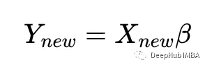
一旦解已知,就可以使用擬合模型計算新的y值給定新的x值,使用:
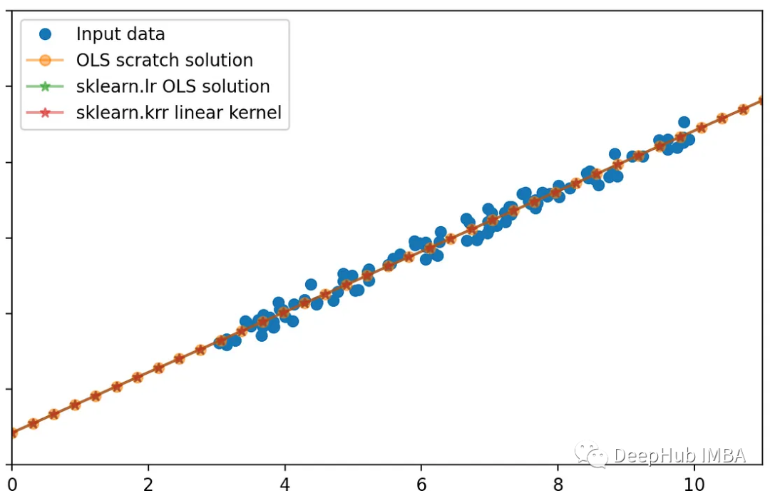
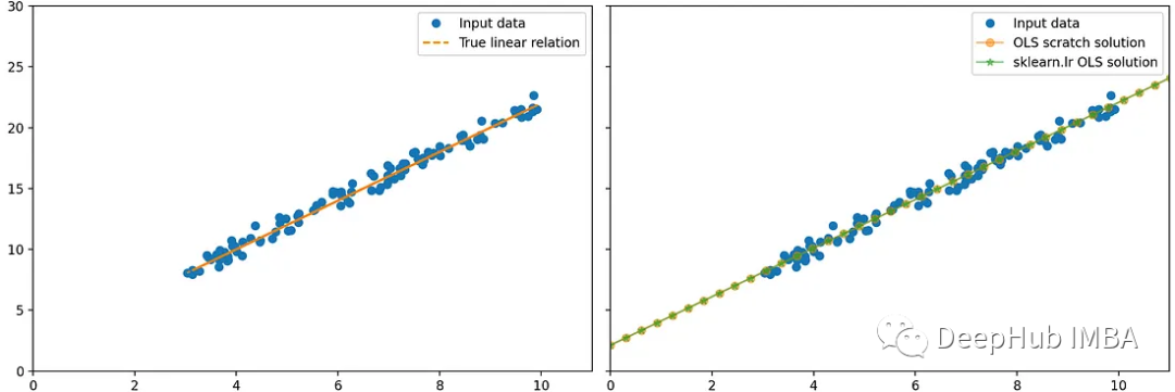
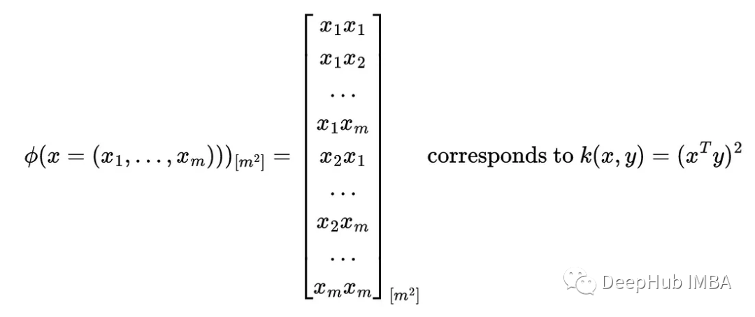
讓我們用scikit-learn來驗證我上面的數學理論:使用sklearn線性回歸器,以及基于numpy的回歸:
%matplotlib qt
 import numpy as np
 import matplotlib.pyplot as plt
 from sklearn.linear_model import LinearRegression

 np.random.seed(0)
 n = 100
 X_ = np.random.uniform(3, 10, n).reshape(-1, 1)
 beta_0 = 2
 beta_1 = 2
 true_y = beta_1 * X_ + beta_0
 noise = np.random.randn(n, 1) * 0.5 # change the scale to reduce/increase noise
 y = true_y + noise

 fig, axes = plt.subplots(1, 2, squeeze=False, sharex=True, sharey=True, figsize=(18, 8))
 axes[0, 0].plot(X_, y, "o", label="Input data")
 axes[0, 0].plot(X_, true_y, '--', label='True linear relation')
 axes[0, 0].set_xlim(0, 11)
 axes[0, 0].set_ylim(0, 30)
 axes[0, 0].legend()

 # f_0 is a column of 1s
 # f_1 is the column of x1
 X = np.c_[np.ones((n, 1)), X_]

 beta_OLS_scratch = np.linalg.inv(X.T @ X) @ X.T @ y
 lr = LinearRegression(
    fit_intercept=False, # do not fit intercept independantly, since we added the 1 column for this purpose
 ).fit(X, y)

 new_X = np.linspace(0, 15, 50).reshape(-1, 1)
 new_X = np.c_[np.ones((50, 1)), new_X]
 new_y_OLS_scratch = new_X @ beta_OLS_scratch
 new_y_lr = lr.predict(new_X)
 axes[0, 1].plot(X_, y, 'o', label='Input data')
 axes[0, 1].plot(new_X[:, 1], new_y_OLS_scratch, '-o', alpha=0.5, label=r"OLS scratch solution")
 axes[0, 1].plot(new_X[:, 1], new_y_lr, '-*', alpha=0.5, label=r"sklearn.lr OLS solution")
 axes[0, 1].legend()
 fig.tight_layout()
 print(beta_OLS_scratch)
 print(lr.coef_)
可以看到,2種方法的結果是相同的
[[2.12458946]
  [1.99549536]]
 [[2.12458946 1.99549536]]
這兩種方法給出了相同的結果
核技巧 Kernel-trick
現在讓我們回顧一種稱為內核技巧的常用技術。
我們最初的問題(可以是任何類似分類或回歸的問題)存在于輸入數據矩陣X的空間中,在m個特征空間中有n個向量的形狀。有時在這個低維空間中,向量不能被分離或分類,所以我們想要將輸入數據轉換到高維空間。可以手工完成,創建新特性。但是隨著特征數量的增長,數值計算也將增加。
核函數的技巧在于使用設計良好的變換函數——通常是T或——從一個長度為m的向量x創建一個長度為m的新向量x ',這樣我們的新數據具有高維數,并且將計算負荷保持在最低限度。
為了達到這個目的,函數必須滿足一些性質,使得新的高維特征空間中的點積可以寫成對應輸入向量的函數——核函數:

這意味著高維空間中的內積可以表示為輸入向量的函數。也就是說我們可以在高維空間中只使用低維向量來計算內積。這就是核技巧:可以從高維空間的通用性中獲益,而無需在那里進行任何計算。
唯一的條件是我們只需要在高維空間中做點積。
實際上有一些強大的數學定理描述了產生這樣的變換和/或這樣的核函數的條件。
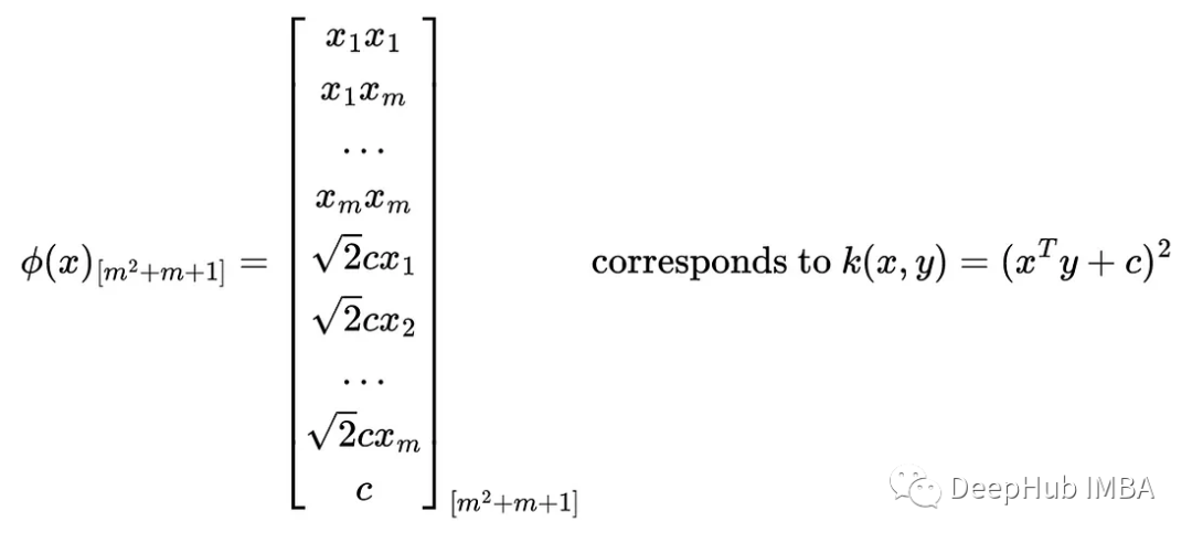
以下是一個核函數示例:
kernel從m維空間創建m^2維空間的第一個例子是使用以下代碼:
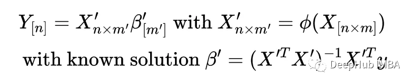
在核函數中添加一個常數會增加維數,其中包含縮放輸入特征的新特征:
下面我們要用到的另一個核函數是線性核函數:

所以恒等變換等價于用一個核函數來計算原始空間的內積。
實際上還有很多其他有用的核,比如徑向核(RBF)核或更一般的多項式核,它們可以創建高維和非線性特征空間。我們這里再簡單介紹一個在線性回歸環境中使用RBF核計算非線性回歸的例子:
import numpy as np
 from sklearn.kernel_ridge import KernelRidge
 import matplotlib.pyplot as plt

 np.random.seed(0)
 X = np.sort(5 * np.random.rand(80, 1), axis=0)
 y = np.sin(X).ravel()
 y[::5] += 3 * (0.5 - np.random.rand(16))

 # Create a test dataset
 X_test = np.arange(0, 5, 0.01)[:, np.newaxis]

 # Fit the KernelRidge model with an RBF kernel
 kr = KernelRidge(
    kernel='rbf', # use RBF kernel
    alpha=1, # regularization
    gamma=1, # scale for rbf
 )
 kr.fit(X, y)

 y_rbf = kr.predict(X_test)

 # Plot the results
 fig, ax = plt.subplots()
 ax.scatter(X, y, color='darkorange', label='Data')
 ax.plot(X_test, y_rbf, color='navy', lw=2, label='RBF Kernel Ridge Regression')
 ax.set_title('Kernel Ridge Regression with RBF Kernel')
 ax.legend()
線性回歸中的線性核
如果變換將x變換為(x)那么我們可以寫出一個新的線性回歸問題
注意維度是如何變化的:線性回歸問題的輸入矩陣從[nxm]變為[nxm '],因此系數向量從長度m變為m '。
這就是核函數的訣竅:當計算解'時,注意到X '與其轉置的乘積出現了,它實際上是所有點積的矩陣,它被稱為核矩陣

線性核化和線性回歸
最后,讓我們看看這個陳述:在線性回歸中使用線性核是無用的,因為它等同于標準線性回歸。
線性核通常用于支持向量機的上下文中,但我想知道它在線性回歸中的表現。
為了證明這兩種方法是等價的,我們必須證明:

使用beta的第一種方法是原始線性回歸,使用beta '的第二種方法是使用線性核化方法。我們可以用上面的矩陣性質和關系來證明這一點:

我們可以使用python和scikit learn再次驗證這一點:
%matplotlib qt
 import numpy as np
 import matplotlib.pyplot as plt
 from sklearn.linear_model import LinearRegression

 np.random.seed(0)
 n = 100
 X_ = np.random.uniform(3, 10, n).reshape(-1, 1)
 beta_0 = 2
 beta_1 = 2
 true_y = beta_1 * X_ + beta_0
 noise = np.random.randn(n, 1) * 0.5 # change the scale to reduce/increase noise
 y = true_y + noise

 fig, axes = plt.subplots(1, 2, squeeze=False, sharex=True, sharey=True, figsize=(18, 8))
 axes[0, 0].plot(X_, y, "o", label="Input data")
 axes[0, 0].plot(X_, true_y, '--', label='True linear relation')
 axes[0, 0].set_xlim(0, 11)
 axes[0, 0].set_ylim(0, 30)
 axes[0, 0].legend()

 # f_0 is a column of 1s
 # f_1 is the column of x1
 X = np.c_[np.ones((n, 1)), X_]

 beta_OLS_scratch = np.linalg.inv(X.T @ X) @ X.T @ y
 lr = LinearRegression(
    fit_intercept=False, # do not fit intercept independantly, since we added the 1 column for this purpose
 ).fit(X, y)

 new_X = np.linspace(0, 15, 50).reshape(-1, 1)
 new_X = np.c_[np.ones((50, 1)), new_X]
 new_y_OLS_scratch = new_X @ beta_OLS_scratch
 new_y_lr = lr.predict(new_X)
 axes[0, 1].plot(X_, y, 'o', label='Input data')
 axes[0, 1].plot(new_X[:, 1], new_y_OLS_scratch, '-o', alpha=0.5, label=r"OLS scratch solution")
 axes[0, 1].plot(new_X[:, 1], new_y_lr, '-*', alpha=0.5, label=r"sklearn.lr OLS solution")
 axes[0, 1].legend()
 fig.tight_layout()
 print(beta_OLS_scratch)
 print(lr.coef_)
總結
在這篇文章中,我們回顧了簡單線性回歸,包括問題的矩陣公式及其解決方案。
然后我們介紹了了核技巧,以及它如何允許我們從高維空間中獲益,并且不需要將低維數據實際移動到這個計算密集型空間。
最后,我證明了線性回歸背景下的線性核實際上是無用的,它對應于簡單的線性回歸。