從 0 開(kāi)始用 PyTorch 構(gòu)建完整的 NeRF
本文經(jīng)自動(dòng)駕駛之心公眾號(hào)授權(quán)轉(zhuǎn)載,轉(zhuǎn)載請(qǐng)聯(lián)系出處。
在解釋代碼之前,首先對(duì)NeRF(神經(jīng)輻射場(chǎng))的原理與含義進(jìn)行簡(jiǎn)單回顧。而NeRF論文中是這樣解釋NeRF算法流程的:
“我們提出了一個(gè)當(dāng)前最優(yōu)的方法,應(yīng)用于復(fù)雜場(chǎng)景下合成新視圖的任務(wù),具體的實(shí)現(xiàn)原理是使用一個(gè)稀疏的輸入視圖集合,然后不斷優(yōu)化底層的連續(xù)體素場(chǎng)景函數(shù)。我們的算法,使用一個(gè)全連接(非卷積)的深度網(wǎng)絡(luò),表示一個(gè)場(chǎng)景,這個(gè)深度網(wǎng)絡(luò)的輸入是一個(gè)單獨(dú)的5D坐標(biāo)(空間位置(x,y,z)和視圖方向(xita,sigma)),其對(duì)應(yīng)的輸出則是體素密度和視圖關(guān)聯(lián)的輻射向量。我們通過(guò)查詢沿著相機(jī)射線的5D坐標(biāo)合成新的場(chǎng)景視圖,以及通過(guò)使用經(jīng)典的體素渲染技術(shù)將輸出顏色和密度投射到圖像中。因?yàn)轶w素渲染具有天然的可變性,所以優(yōu)化我們的表示方法所需的唯一輸入就是一組已知相機(jī)位姿的圖像。我們介紹如何高效優(yōu)化神經(jīng)輻射場(chǎng)照度,以渲染具有復(fù)雜幾何形狀和外觀的逼真新穎視圖,并展示了由于之前神經(jīng)渲染和視圖合成工作的結(jié)果。”

▲圖1|NeRF實(shí)現(xiàn)流程??【深藍(lán)AI】
基于前文的原理,本節(jié)開(kāi)始講述具體的代碼實(shí)現(xiàn)。首先,導(dǎo)入算法需要的Python庫(kù)文件。
import os
from typing import Optional,Tuple,List,Union,Callable

import numpy as np
import torch
from torch import nn
import matplotlib.pyplot as plt
from mpl_toolkits.mplot3d import axes3d
from tqdm import trange

# 設(shè)置GPU還是CPU設(shè)備
device = torch.device('cuda' if torch.cuda.is_available() else 'cpu')
1 輸入
根據(jù)相關(guān)論文中的介紹可知,NeRF的輸入是一個(gè)包含空間位置坐標(biāo)與視圖方向的5D坐標(biāo)。然而,在PyTorch構(gòu)建NeRF過(guò)程中使用的數(shù)據(jù)集只是一般的3D到2D圖像數(shù)據(jù)集,包含拍攝相機(jī)的內(nèi)參:位姿和焦距。因此在后面的操作中,我們會(huì)把輸入數(shù)據(jù)集轉(zhuǎn)為算法模型需要的輸入形式。
在這一流程中使用樂(lè)高推土機(jī)圖像作為簡(jiǎn)單NeRF算法的數(shù)據(jù)集,如圖2所示:(具體的數(shù)據(jù)鏈接請(qǐng)?jiān)谖哪┎榭矗?/span>

▲圖2|樂(lè)高推土機(jī)數(shù)據(jù)集??【深藍(lán)AI】
這項(xiàng)工作中使用的小型樂(lè)高數(shù)據(jù)集由 106 幅樂(lè)高推土機(jī)的圖像組成,并配有位姿數(shù)據(jù)和常用焦距數(shù)值。與其他數(shù)據(jù)集一樣,這里保留前 100 張圖像用于訓(xùn)練,并保留一張測(cè)試圖像用于驗(yàn)證,具體的加載數(shù)據(jù)操作如下:
data = np.load('tiny_nerf_data.npz') # 加載數(shù)據(jù)集
images = data['images']  # 圖像數(shù)據(jù)
poses = data['poses']  # 位姿數(shù)據(jù)
focal = data['focal']  # 焦距數(shù)值

print(f'Images shape: {images.shape}')
print(f'Poses shape: {poses.shape}')
print(f'Focal length: {focal}')

height, width = images.shape[1:3]
near, far = 2., 6.

n_training = 100 # 訓(xùn)練數(shù)據(jù)數(shù)量
testimg_idx = 101 # 測(cè)試數(shù)據(jù)下標(biāo)
testimg, testpose = images[testimg_idx], poses[testimg_idx]

plt.imshow(testimg)
print('Pose')
print(testpose)
2 數(shù)據(jù)處理
回顧NeRF相關(guān)論文,本次代碼實(shí)現(xiàn)需要的輸入是一個(gè)單獨(dú)的5D坐標(biāo)(空間位置和視圖方向)。因此,我們需要針對(duì)上面使用的小型樂(lè)高數(shù)據(jù)做一個(gè)處理操作。
一般而言,為了收集這些特點(diǎn)輸入數(shù)據(jù),算法中需要對(duì)輸入圖像進(jìn)行反渲染操作。具體來(lái)講就是通過(guò)每個(gè)像素點(diǎn)在三維空間中繪制投影線,并從中提取樣本。
要從圖像以外的三維空間采樣輸入數(shù)據(jù)點(diǎn),首先就得從樂(lè)高照片集中獲取每臺(tái)相機(jī)的初始位姿,然后通過(guò)一些矢量數(shù)學(xué)運(yùn)算,將這些4x4姿態(tài)矩陣轉(zhuǎn)換成「表示原點(diǎn)的三維坐標(biāo)和表示方向的三維矢量」——這兩類信息最終會(huì)結(jié)合起來(lái)描述一個(gè)矢量,該矢量用以表征拍攝照片時(shí)相機(jī)的指向。
下列代碼則正是通過(guò)繪制箭頭來(lái)描述這一操作,箭頭表示每一幀圖像的原點(diǎn)和方向:
# 方向數(shù)據(jù)
dirs = np.stack([np.sum([0, 0, -1] * pose[:3, :3], axis=-1) for pose in poses])
# 原點(diǎn)數(shù)據(jù)
origins = poses[:, :3, -1]

# 繪圖的設(shè)置

ax = plt.figure(figsize=(12, 8)).add_subplot(projectinotallow='3d')
_ = ax.quiver(
  origins[..., 0].flatten(),
  origins[..., 1].flatten(),
  origins[..., 2].flatten(),
  dirs[..., 0].flatten(),
  dirs[..., 1].flatten(),
  dirs[..., 2].flatten(), length=0.5, normalize=True)

ax.set_xlabel('X')

ax.set_ylabel('Y')

ax.set_zlabel('z')

plt.show()
最終繪制出來(lái)的箭頭結(jié)果如下圖所示:

▲圖3|采樣點(diǎn)相機(jī)拍攝指向??【深藍(lán)AI】
當(dāng)有了這些相機(jī)位姿數(shù)據(jù)之后,我們就可以沿著圖像的每個(gè)像素找到投影線,而每條投影線都是由其原點(diǎn)(x,y,z)和方向聯(lián)合定義。其中每個(gè)像素的原點(diǎn)可能相同,但方向一般是不同的。這些方向射線都略微偏離中心,因此不會(huì)存在兩條平行方向線,如下圖所示:

根據(jù)圖4所述的原理,我們就可以確定每條射線的方向和原點(diǎn),相關(guān)代碼如下:
def get_rays(
  height: int, # 圖像高度
  width: int, # 圖像寬帶
  focal_length: float, # 焦距
  c2w: torch.Tensor
) -> Tuple[torch.Tensor, torch.Tensor]:
  """
  通過(guò)每個(gè)像素和相機(jī)原點(diǎn),找到射線的原點(diǎn)和方向。

 """


  # 應(yīng)用針孔相機(jī)模型收集每個(gè)像素的方向
  i, j = torch.meshgrid(
      torch.arange(width, dtype=torch.float32).to(c2w),
      torch.arange(height, dtype=torch.float32).to(c2w),
      indexing='ij')

  i, j = i.transpose(-1, -2), j.transpose(-1, -2)

  # 方向數(shù)據(jù)
  directions = torch.stack([(i - width * .5) / focal_length,
                            -(j - height * .5) / focal_length,
                            -torch.ones_like(i)
                           ], dim=-1)


  # 用相機(jī)位姿求出方向
  rays_d = torch.sum(directions[..., None, :] * c2w[:3, :3], dim=-1)


  # 默認(rèn)所有射線原點(diǎn)相同
  rays_o = c2w[:3, -1].expand(rays_d.shape)
  return rays_o, rays_d
得到每個(gè)像素對(duì)應(yīng)的射線的方向數(shù)據(jù)和原點(diǎn)數(shù)據(jù)之后,就能夠獲得了NeRF算法中需要的五維數(shù)據(jù)輸入,下面將這些數(shù)據(jù)調(diào)整為算法輸入的格式:
# 轉(zhuǎn)為PyTorch的tensor
images = torch.from_numpy(data['images'][:n_training]).to(device)
poses = torch.from_numpy(data['poses']).to(device)
focal = torch.from_numpy(data['focal']).to(device)
testimg = torch.from_numpy(data['images'][testimg_idx]).to(device)
testpose = torch.from_numpy(data['poses'][testimg_idx]).to(device)


# 針對(duì)每個(gè)圖像獲取射線
height, width = images.shape[1:3]

with torch.no_grad():
  ray_origin, ray_direction = get_rays(height, width, focal, testpose)


print('Ray Origin')

print(ray_origin.shape)
print(ray_origin[height // 2, width // 2, :])
print('')


print('Ray Direction')

print(ray_direction.shape)
print(ray_direction[height // 2, width // 2, :])
print('')
分層采樣
當(dāng)算法輸入模塊有了NeRF算法需要的輸入數(shù)據(jù),也就是包含原點(diǎn)和方向向量組合的線條時(shí),就可以在線條上進(jìn)行采樣。這一過(guò)程是采用從粗到細(xì)的采樣策略,即分層采樣策略。
具體來(lái)說(shuō),分層采樣就是將光線分成均勻分布的小塊,接著在每個(gè)小塊內(nèi)隨機(jī)抽樣。其中擾動(dòng)的設(shè)置決定了是均勻取樣的,還是直接簡(jiǎn)單使用分區(qū)中心作為采樣點(diǎn)。具體操作代碼如下所示:
# 采樣函數(shù)定義
def sample_stratified(
  rays_o: torch.Tensor, # 射線原點(diǎn)
  rays_d: torch.Tensor, # 射線方向
  near: float,
  far: float,
  n_samples: int, # 采樣數(shù)量
  perturb: Optional[bool] = True, # 擾動(dòng)設(shè)置
  inverse_depth: bool = False  # 反向深度
) -> Tuple[torch.Tensor, torch.Tensor]:
  """
  從規(guī)則的bin中沿著射線進(jìn)行采樣。
  """

  # 沿著射線抓取采樣點(diǎn)
  t_vals = torch.linspace(0., 1., n_samples, device=rays_o.device)
  if not inverse_depth:
    # 由遠(yuǎn)到近線性采樣
    z_vals = near * (1.-t_vals) + far * (t_vals)
  else:
    # 在反向深度中線性采樣
  z_vals = 1./(1./near * (1.-t_vals) + 1./far * (t_vals))

  # 沿著射線從bins中統(tǒng)一采樣
  if perturb:
    mids = .5 * (z_vals[1:] + z_vals[:-1])
    upper = torch.concat([mids, z_vals[-1:]], dim=-1)
    lower = torch.concat([z_vals[:1], mids], dim=-1)
    t_rand = torch.rand([n_samples], device=z_vals.device)
    z_vals = lower + (upper - lower) * t_rand
  z_vals = z_vals.expand(list(rays_o.shape[:-1]) + [n_samples])

  # 應(yīng)用相應(yīng)的縮放參數(shù)
  pts = rays_o[..., None, :] + rays_d[..., None, :] * z_vals[..., :, None]
  return pts, z_vals
接著就到了對(duì)這些采樣點(diǎn)做可視化分析的步驟。如圖5中所述,未受擾動(dòng)的藍(lán) 色點(diǎn)是bin的“中心“,而紅點(diǎn)對(duì)應(yīng)擾動(dòng)點(diǎn)的采樣。請(qǐng)注意,紅點(diǎn)與上方的藍(lán)點(diǎn)略有偏移,但所有點(diǎn)都在遠(yuǎn)近采樣設(shè)定值之間。具體代碼如下:
y_vals = torch.zeros_like(z_vals)
# 調(diào)用采樣策略函數(shù)
_, z_vals_unperturbed = sample_stratified(rays_o, rays_d, near, far, n_samples,
                                  perturb=False, inverse_depth=inverse_depth)
# 繪圖相關(guān)plt.plot(z_vals_unperturbed[0].cpu().numpy(), 1 + y_vals[0].cpu().numpy(), 'b-o')
plt.plot(z_vals[0].cpu().numpy(), y_vals[0].cpu().numpy(), 'r-o')
plt.ylim([-1, 2])
plt.title('Stratified Sampling (blue) with Perturbation (red)')
ax = plt.gca()
ax.axes.yaxis.set_visible(False)
plt.grid(True)
▲圖5|采樣結(jié)果示意圖??【深藍(lán)AI】
3 位置編碼
與Transformer一樣,NeRF也使用了位置編碼器。因此NeRF就需要借助位置編碼器將輸入映射到更高的頻率空間,以彌補(bǔ)神經(jīng)網(wǎng)絡(luò)在學(xué)習(xí)低頻函數(shù)時(shí)的偏差。
這一環(huán)節(jié)將會(huì)為位置編碼器建立一個(gè)簡(jiǎn)單的 torch.nn.Module 模塊,相同的編碼器可同時(shí)用于對(duì)輸入樣本和視圖方向的編碼操作。注意,這些輸入被指定了不同的參數(shù)。代碼如下所示:
# 位置編碼類
class PositionalEncoder(nn.Module):
  """
  對(duì)輸入點(diǎn),做sine或者consine位置編碼。
  """
  def __init__(
    self,
    d_input: int,
    n_freqs: int,
    log_space: bool = False
  ):
    super().__init__()
    self.d_input = d_input
    self.n_freqs = n_freqs
    self.log_space = log_space
    self.d_output = d_input * (1 + 2 * self.n_freqs)
    self.embed_fns = [lambda x: x]

    # 定義線性或者log尺度的頻率
    if self.log_space:
      freq_bands = 2.**torch.linspace(0., self.n_freqs - 1, self.n_freqs)
    else:
      freq_bands = torch.linspace(2.**0., 2.**(self.n_freqs - 1), self.n_freqs)

    # 替換sin和cos
    for freq in freq_bands:
      self.embed_fns.append(lambda x, freq=freq: torch.sin(x * freq))
      self.embed_fns.append(lambda x, freq=freq: torch.cos(x * freq))

  def forward(
    self,
    x
  ) -> torch.Tensor:
    """
    實(shí)際使用位置編碼的函數(shù)。
    """
    return torch.concat([fn(x) for fn in self.embed_fns], dim=-1)
4 NeRF模型
在此,定義一個(gè)NeRF 模型——主要由線性層模塊列表構(gòu)成,而列表中進(jìn)一步包含非線性激活函數(shù)和殘差連接。該模型有一個(gè)可選的視圖方向輸入,如果在實(shí)例化時(shí)提供具體的方向信息,那么會(huì)改變模型結(jié)構(gòu)。
(本實(shí)現(xiàn)基于原始論文NeRF:Representing Scenes as Neural Radiance Fields for View Synthesis 的第3節(jié),并使用相同的默認(rèn)設(shè)置)
具體代碼如下所示:
# 定義NeRF模型
class NeRF(nn.Module):
  """
  神經(jīng)輻射場(chǎng)模塊。
  """
  def __init__(
    self,
    d_input: int = 3,
    n_layers: int = 8,
    d_filter: int = 256,
    skip: Tuple[int] = (4,),
    d_viewdirs: Optional[int] = None
  ):
    super().__init__()
    self.d_input = d_input # 輸入
    self.skip = skip # 殘差連接
    self.act = nn.functional.relu # 激活函數(shù)
    self.d_viewdirs = d_viewdirs # 視圖方向

    # 創(chuàng)建模型的層結(jié)構(gòu)
    self.layers = nn.ModuleList(
      [nn.Linear(self.d_input, d_filter)] +
      [nn.Linear(d_filter + self.d_input, d_filter) if i in skip \
       else nn.Linear(d_filter, d_filter) for i in range(n_layers - 1)]
    )

    # Bottleneck 層
    if self.d_viewdirs is not None:
      # 如果使用視圖方向,分離alpha和RGB
      self.alpha_out = nn.Linear(d_filter, 1)
      self.rgb_filters = nn.Linear(d_filter, d_filter)
      self.branch = nn.Linear(d_filter + self.d_viewdirs, d_filter // 2)
      self.output = nn.Linear(d_filter // 2, 3)
    else:
      # 如果不使用試圖方向,則簡(jiǎn)單輸出
      self.output = nn.Linear(d_filter, 4)

  def forward(
    self,
    x: torch.Tensor,
    viewdirs: Optional[torch.Tensor] = None
  ) -> torch.Tensor:
    r"""
    帶有視圖方向的前向傳播
    """

    # 判斷是否設(shè)置視圖方向
    if self.d_viewdirs is None and viewdirs is not None:
      raise ValueError('Cannot input x_direction if d_viewdirs was not given.')

    # 運(yùn)行bottleneck層之前的網(wǎng)絡(luò)層
    x_input = x
    for i, layer in enumerate(self.layers):
      x = self.act(layer(x))
      if i in self.skip:
        x = torch.cat([x, x_input], dim=-1)

    # 運(yùn)行 bottleneck
    if self.d_viewdirs is not None:
      # Split alpha from network output
      alpha = self.alpha_out(x)

      # 結(jié)果傳入到rgb過(guò)濾器
      x = self.rgb_filters(x)
      x = torch.concat([x, viewdirs], dim=-1)
      x = self.act(self.branch(x))
      x = self.output(x)

      # 拼接alpha一起作為輸出
      x = torch.concat([x, alpha], dim=-1)
    else:
      # 不拼接,簡(jiǎn)單輸出
      x = self.output(x)
    return x
5 體積渲染
上面得到NeRF模型的輸出結(jié)果之后,仍需將NeRF的輸出轉(zhuǎn)換成圖像。也就是通過(guò)渲染模塊對(duì)每個(gè)像素沿光線方向的所有樣本進(jìn)行加權(quán)求和,從而得到該像素的估計(jì)顏色值,此外每個(gè)RGB樣本都會(huì)根據(jù)其Alpha值進(jìn)行加權(quán)。其中Alpha值越高,表明采樣區(qū)域不透明的可能性越大,因此沿射線方向越遠(yuǎn)的點(diǎn)越有可能被遮擋,累加乘積可確保更遠(yuǎn)處的點(diǎn)受到抑制。具體代碼如下:
# 體積渲染
def cumprod_exclusive(
  tensor: torch.Tensor
) -> torch.Tensor:
  """
  (Courtesy of https://github.com/krrish94/nerf-pytorch)

  和tf.math.cumprod(..., exclusive=True)功能類似

  參數(shù):
  tensor (torch.Tensor): Tensor whose cumprod (cumulative product, see `torch.cumprod`) along dim=-1
    is to be computed.
  返回值:
  cumprod (torch.Tensor): cumprod of Tensor along dim=-1, mimiciking the functionality of
    tf.math.cumprod(..., exclusive=True) (see `tf.math.cumprod` for details).
  """

  # 首先計(jì)算規(guī)則的cunprod
  cumprod = torch.cumprod(tensor, -1)
  cumprod = torch.roll(cumprod, 1, -1)
  # 用1替換首個(gè)元素
  cumprod[..., 0] = 1.

  return cumprod

# 輸出到圖像的函數(shù)
def raw2outputs(
  raw: torch.Tensor,
  z_vals: torch.Tensor,
  rays_d: torch.Tensor,
  raw_noise_std: float = 0.0,
  white_bkgd: bool = False
) -> Tuple[torch.Tensor, torch.Tensor, torch.Tensor, torch.Tensor]:
  """
  將NeRF的輸出轉(zhuǎn)換為RGB輸出。
  """

  # 沿著`z_vals`軸元素之間的差值.
  dists = z_vals[..., 1:] - z_vals[..., :-1]
  dists = torch.cat([dists, 1e10 * torch.ones_like(dists[..., :1])], dim=-1)

  # 將每個(gè)距離乘以相應(yīng)方向射線的法線,轉(zhuǎn)換為現(xiàn)實(shí)世界中的距離(考慮非單位方向)。
  dists = dists * torch.norm(rays_d[..., None, :], dim=-1)

  # 為模型預(yù)測(cè)密度添加噪音。可用于在訓(xùn)練過(guò)程中對(duì)網(wǎng)絡(luò)進(jìn)行正則化(防止出現(xiàn)浮點(diǎn)偽影)。
  noise = 0.
  if raw_noise_std > 0.:
    noise = torch.randn(raw[..., 3].shape) * raw_noise_std

  # Predict density of each sample along each ray. Higher values imply
  # higher likelihood of being absorbed at this point. [n_rays, n_samples]
  alpha = 1.0 - torch.exp(-nn.functional.relu(raw[..., 3] + noise) * dists)

  # 預(yù)測(cè)每條射線上每個(gè)樣本的密度。數(shù)值越大,表示該點(diǎn)被吸收的可能性越大。[n_ 射線,n_樣本]
  weights = alpha * cumprod_exclusive(1. - alpha + 1e-10)

  # 計(jì)算RGB圖的權(quán)重。
  rgb = torch.sigmoid(raw[..., :3])  # [n_rays, n_samples, 3]
  rgb_map = torch.sum(weights[..., None] * rgb, dim=-2)  # [n_rays, 3]

  # 估計(jì)預(yù)測(cè)距離的深度圖。
  depth_map = torch.sum(weights * z_vals, dim=-1)

  # 稀疏圖
  disp_map = 1. / torch.max(1e-10 * torch.ones_like(depth_map),
                            depth_map / torch.sum(weights, -1))

  # 沿著每條射線加權(quán)。
  acc_map = torch.sum(weights, dim=-1)

  # 要合成到白色背景上,請(qǐng)使用累積的 alpha 貼圖。
  if white_bkgd:
    rgb_map = rgb_map + (1. - acc_map[..., None])

  return rgb_map, depth_map, acc_map, weights
6 分層體積采樣
事實(shí)上,三維空間中的遮擋物非常稀疏,因此大多數(shù)點(diǎn)對(duì)渲染圖像的貢獻(xiàn)不大。所以,對(duì)積分有貢獻(xiàn)的區(qū)域進(jìn)行超采樣會(huì)有更好的效果。這里,筆者對(duì)第一組樣本應(yīng)用基于歸一化的權(quán)重來(lái)創(chuàng)建整個(gè)光線的概率密度函數(shù),然后對(duì)該密度函數(shù)應(yīng)用反變換采樣來(lái)收集第二組樣本。具體代碼如下:
# 采樣概率密度函數(shù)
def sample_pdf(
  bins: torch.Tensor,
  weights: torch.Tensor,
  n_samples: int,
  perturb: bool = False
) -> torch.Tensor:
  """
  應(yīng)用反向轉(zhuǎn)換采樣到一組加權(quán)點(diǎn)。
  """

  # 正則化權(quán)重得到概率密度函數(shù)。
  pdf = (weights + 1e-5) / torch.sum(weights + 1e-5, -1, keepdims=True) # [n_rays, weights.shape[-1]]

  # 將概率密度函數(shù)轉(zhuǎn)為累計(jì)分布函數(shù)。
  cdf = torch.cumsum(pdf, dim=-1) # [n_rays, weights.shape[-1]]
  cdf = torch.concat([torch.zeros_like(cdf[..., :1]), cdf], dim=-1) # [n_rays, weights.shape[-1] + 1]

  # 從累計(jì)分布函數(shù)中提取樣本位置。perturb == 0 時(shí)為線性。
  if not perturb:
    u = torch.linspace(0., 1., n_samples, device=cdf.device)
    u = u.expand(list(cdf.shape[:-1]) + [n_samples]) # [n_rays, n_samples]
  else:
    u = torch.rand(list(cdf.shape[:-1]) + [n_samples], device=cdf.device) # [n_rays, n_samples]

  # 沿累計(jì)分布函數(shù)找出 u 值所在的索引。
  u = u.contiguous() # 返回具有相同值的連續(xù)張量。
  inds = torch.searchsorted(cdf, u, right=True) # [n_rays, n_samples]

  # 夾住超出范圍的索引。
  below = torch.clamp(inds - 1, min=0)
  above = torch.clamp(inds, max=cdf.shape[-1] - 1)
  inds_g = torch.stack([below, above], dim=-1) # [n_rays, n_samples, 2]

  # 從累計(jì)分布函數(shù)和相應(yīng)的 bin 中心取樣。
  matched_shape = list(inds_g.shape[:-1]) + [cdf.shape[-1]]
  cdf_g = torch.gather(cdf.unsqueeze(-2).expand(matched_shape), dim=-1,
                       index=inds_g)
  bins_g = torch.gather(bins.unsqueeze(-2).expand(matched_shape), dim=-1,
                        index=inds_g)

  # 將樣本轉(zhuǎn)換為射線長(zhǎng)度。
  denom = (cdf_g[..., 1] - cdf_g[..., 0])
  denom = torch.where(denom < 1e-5, torch.ones_like(denom), denom)
  t = (u - cdf_g[..., 0]) / denom
  samples = bins_g[..., 0] + t * (bins_g[..., 1] - bins_g[..., 0])

  return samples # [n_rays, n_samples]
7 整體的前向傳播流程
此時(shí)應(yīng)將上面所有內(nèi)容整合在一起,通過(guò)模型計(jì)算一次前向傳遞。
由于潛在的內(nèi)存問(wèn)題,前向傳遞以“塊“為單位進(jìn)行計(jì)算,然后匯總到一個(gè)批次中。梯度傳播是在整個(gè)批次處理完畢后進(jìn)行的,因此有“塊“和“批次“之分。對(duì)于內(nèi)存緊張環(huán)境來(lái)說(shuō),分塊處理尤為重要,因?yàn)樵摥h(huán)境下提供的資源比原始論文中引用的資源更為有限。具體代碼如下所示:
def get_chunks(
  inputs: torch.Tensor,
  chunksize: int = 2**15
) -> List[torch.Tensor]:
  """
  輸入分塊。
  """
  return [inputs[i:i + chunksize] for i in range(0, inputs.shape[0], chunksize)]

def prepare_chunks(
  points: torch.Tensor,
  encoding_function: Callable[[torch.Tensor], torch.Tensor],
  chunksize: int = 2**15
) -> List[torch.Tensor]:
  """
  對(duì)點(diǎn)進(jìn)行編碼和分塊,為 NeRF 模型做好準(zhǔn)備。
  """
  points = points.reshape((-1, 3))
  points = encoding_function(points)
  points = get_chunks(points, chunksize=chunksize)
  return points

def prepare_viewdirs_chunks(
  points: torch.Tensor,
  rays_d: torch.Tensor,
  encoding_function: Callable[[torch.Tensor], torch.Tensor],
  chunksize: int = 2**15
) -> List[torch.Tensor]:
  r"""
  對(duì)視圖方向進(jìn)行編碼和分塊,為 NeRF 模型做好準(zhǔn)備。
  """
  viewdirs = rays_d / torch.norm(rays_d, dim=-1, keepdim=True)
  viewdirs = viewdirs[:, None, ...].expand(points.shape).reshape((-1, 3))
  viewdirs = encoding_function(viewdirs)
  viewdirs = get_chunks(viewdirs, chunksize=chunksize)
  return viewdirs
def nerf_forward(
  rays_o: torch.Tensor,
  rays_d: torch.Tensor,
  near: float,
  far: float,
  encoding_fn: Callable[[torch.Tensor], torch.Tensor],
  coarse_model: nn.Module,
  kwargs_sample_stratified: dict = None,
  n_samples_hierarchical: int = 0,
  kwargs_sample_hierarchical: dict = None,
  fine_model = None,
  viewdirs_encoding_fn: Optional[Callable[[torch.Tensor], torch.Tensor]] = None,
  chunksize: int = 2**15
) -> Tuple[torch.Tensor, torch.Tensor, torch.Tensor, dict]:
  """
  計(jì)算一次前向傳播
  """

  # 設(shè)置參數(shù)
  if kwargs_sample_stratified is None:
    kwargs_sample_stratified = {}
  if kwargs_sample_hierarchical is None:
    kwargs_sample_hierarchical = {}

  # 沿著每條射線的樣本查詢點(diǎn)。
  query_points, z_vals = sample_stratified(
      rays_o, rays_d, near, far, **kwargs_sample_stratified)

  # 準(zhǔn)備批次。
  batches = prepare_chunks(query_points, encoding_fn, chunksize=chunksize)
  if viewdirs_encoding_fn is not None:
    batches_viewdirs = prepare_viewdirs_chunks(query_points, rays_d,
                                               viewdirs_encoding_fn,
                                               chunksize=chunksize)
  else:
    batches_viewdirs = [None] * len(batches)

  # 稀疏模型流程。
  predictions = []
  for batch, batch_viewdirs in zip(batches, batches_viewdirs):
    predictions.append(coarse_model(batch, viewdirs=batch_viewdirs))
  raw = torch.cat(predictions, dim=0)
  raw = raw.reshape(list(query_points.shape[:2]) + [raw.shape[-1]])

  # 執(zhí)行可微分體積渲染,重新合成 RGB 圖像。
  rgb_map, depth_map, acc_map, weights = raw2outputs(raw, z_vals, rays_d)

  outputs = {
      'z_vals_stratified': z_vals
  }

  if n_samples_hierarchical > 0:
    # Save previous outputs to return.
    rgb_map_0, depth_map_0, acc_map_0 = rgb_map, depth_map, acc_map

    # 對(duì)精細(xì)查詢點(diǎn)進(jìn)行分層抽樣。
    query_points, z_vals_combined, z_hierarch = sample_hierarchical(
      rays_o, rays_d, z_vals, weights, n_samples_hierarchical,
      **kwargs_sample_hierarchical)

    # 像以前一樣準(zhǔn)備輸入。
    batches = prepare_chunks(query_points, encoding_fn, chunksize=chunksize)
    if viewdirs_encoding_fn is not None:
      batches_viewdirs = prepare_viewdirs_chunks(query_points, rays_d,
                                                 viewdirs_encoding_fn,
                                                 chunksize=chunksize)
    else:
      batches_viewdirs = [None] * len(batches)

    # 通過(guò)精細(xì)模型向前傳遞新樣本。
    fine_model = fine_model if fine_model is not None else coarse_model
    predictions = []
    for batch, batch_viewdirs in zip(batches, batches_viewdirs):
      predictions.append(fine_model(batch, viewdirs=batch_viewdirs))
    raw = torch.cat(predictions, dim=0)
    raw = raw.reshape(list(query_points.shape[:2]) + [raw.shape[-1]])

    # 執(zhí)行可微分體積渲染,重新合成 RGB 圖像。
    rgb_map, depth_map, acc_map, weights = raw2outputs(raw, z_vals_combined, rays_d)

    # 存儲(chǔ)輸出
    outputs['z_vals_hierarchical'] = z_hierarch
    outputs['rgb_map_0'] = rgb_map_0
    outputs['depth_map_0'] = depth_map_0
    outputs['acc_map_0'] = acc_map_0

  # 存儲(chǔ)輸出
  outputs['rgb_map'] = rgb_map
  outputs['depth_map'] = depth_map
  outputs['acc_map'] = acc_map
  outputs['weights'] = weights
  return outputs
到這一步驟,就幾乎擁有了訓(xùn)練模型所需的一切模塊。現(xiàn)在為一個(gè)簡(jiǎn)單的訓(xùn)練過(guò)程做一些設(shè)置,創(chuàng)建超參數(shù)和輔助函數(shù),然后來(lái)訓(xùn)練模型。
7.1 超參數(shù)
所有用于訓(xùn)練的超參數(shù)都在此設(shè)置,默認(rèn)值取自原始論文中數(shù)據(jù),除非計(jì)算上有限制。在計(jì)算受限情況下,本次討論采用的都是合理的默認(rèn)值。
# 編碼器
d_input = 3           # 輸入維度
n_freqs = 10          # 輸入到編碼函數(shù)中的樣本點(diǎn)數(shù)量
log_space = True      # 如果設(shè)置,頻率按對(duì)數(shù)空間縮放
use_viewdirs = True   # 如果設(shè)置,則使用視圖方向作為輸入
n_freqs_views = 4     # 視圖編碼功能的數(shù)量

# 采樣策略
n_samples = 64         # 每條射線的空間樣本數(shù)
perturb = True         # 如果設(shè)置,則對(duì)采樣位置應(yīng)用噪聲
inverse_depth = False  # 如果設(shè)置,則按反深度線性采樣點(diǎn)

# 模型
d_filter = 128          # 線性層濾波器的尺寸
n_layers = 2            # bottleneck層數(shù)量
skip = []               # 應(yīng)用輸入殘差的層級(jí)
use_fine_model = True   # 如果設(shè)置,則創(chuàng)建一個(gè)精細(xì)模型
d_filter_fine = 128     # 精細(xì)網(wǎng)絡(luò)線性層濾波器的尺寸
n_layers_fine = 6       # 精細(xì)網(wǎng)絡(luò)瓶頸層數(shù)

# 分層采樣
n_samples_hierarchical = 64   # 每條射線的樣本數(shù)
perturb_hierarchical = False  # 如果設(shè)置,則對(duì)采樣位置應(yīng)用噪聲

# 優(yōu)化器
lr = 5e-4  # 學(xué)習(xí)率

# 訓(xùn)練
n_iters = 10000
batch_size = 2**14          # 每個(gè)梯度步長(zhǎng)的射線數(shù)量(2 的冪次)
one_image_per_step = True   # 每個(gè)梯度步驟一個(gè)圖像(禁用批處理)
chunksize = 2**14           # 根據(jù)需要進(jìn)行修改,以適應(yīng) GPU 內(nèi)存
center_crop = True          # 裁剪圖像的中心部分(每幅圖像裁剪一次)
center_crop_iters = 50      # 經(jīng)過(guò)這么多epoch后,停止裁剪中心
display_rate = 25          # 每 X 個(gè)epoch顯示一次測(cè)試輸出

# 早停
warmup_iters = 100          # 熱身階段的迭代次數(shù)
warmup_min_fitness = 10.0   # 在熱身_iters 處繼續(xù)訓(xùn)練的最小 PSNR 值
n_restarts = 10             # 訓(xùn)練停滯時(shí)重新開(kāi)始的次數(shù)

# 捆綁了各種函數(shù)的參數(shù),以便一次性傳遞。
kwargs_sample_stratified = {
    'n_samples': n_samples,
    'perturb': perturb,
    'inverse_depth': inverse_depth
}
kwargs_sample_hierarchical = {
    'perturb': perturb
}
7.2 訓(xùn)練類和函數(shù)
這一環(huán)節(jié)會(huì)創(chuàng)建一些用于訓(xùn)練的輔助函數(shù)。NeRF很容易出現(xiàn)局部最小值,在這種情況下,訓(xùn)練很快就會(huì)停滯并產(chǎn)生空白輸出。必要時(shí),會(huì)利用EarlyStopping重新啟動(dòng)訓(xùn)練。
# 繪制采樣函數(shù)
def plot_samples(
  z_vals: torch.Tensor,
  z_hierarch: Optional[torch.Tensor] = None,
  ax: Optional[np.ndarray] = None):
  r"""
  繪制分層樣本和(可選)分級(jí)樣本。
  """
  y_vals = 1 + np.zeros_like(z_vals)

  if ax is None:
    ax = plt.subplot()
  ax.plot(z_vals, y_vals, 'b-o')
  if z_hierarch is not None:
    y_hierarch = np.zeros_like(z_hierarch)
    ax.plot(z_hierarch, y_hierarch, 'r-o')
  ax.set_ylim([-1, 2])
  ax.set_title('Stratified  Samples (blue) and Hierarchical Samples (red)')
  ax.axes.yaxis.set_visible(False)
  ax.grid(True)
  return ax

def crop_center(
  img: torch.Tensor,
  frac: float = 0.5
) -> torch.Tensor:
  r"""
  從圖像中裁剪中心方形。
  """
  h_offset = round(img.shape[0] * (frac / 2))
  w_offset = round(img.shape[1] * (frac / 2))
  return img[h_offset:-h_offset, w_offset:-w_offset]

class EarlyStopping:
  r"""
  基于適配標(biāo)準(zhǔn)的早期停止輔助器
  """
  def __init__(
    self,
    patience: int = 30,
    margin: float = 1e-4
  ):
    self.best_fitness = 0.0
    self.best_iter = 0
    self.margin = margin
    self.patience = patience or float('inf')  # 在epoch停止提高后等待的停止時(shí)間

  def __call__(
    self,
    iter: int,
    fitness: float
  ):
    r"""
    檢查是否符合停止標(biāo)準(zhǔn)。
    """
    if (fitness - self.best_fitness) > self.margin:
      self.best_iter = iter
      self.best_fitness = fitness
    delta = iter - self.best_iter
    stop = delta >= self.patience  # 超過(guò)耐性則停止訓(xùn)練
    return stop
def init_models():
  r"""
  為 NeRF 訓(xùn)練初始化模型、編碼器和優(yōu)化器。
  """
  # 編碼器
  encoder = PositionalEncoder(d_input, n_freqs, log_space=log_space)
  encode = lambda x: encoder(x)

  # 視圖方向編碼
  if use_viewdirs:
    encoder_viewdirs = PositionalEncoder(d_input, n_freqs_views,
                                        log_space=log_space)
    encode_viewdirs = lambda x: encoder_viewdirs(x)
    d_viewdirs = encoder_viewdirs.d_output
  else:
    encode_viewdirs = None
    d_viewdirs = None

  # 模型
  model = NeRF(encoder.d_output, n_layers=n_layers, d_filter=d_filter, skip=skip,
              d_viewdirs=d_viewdirs)
  model.to(device)
  model_params = list(model.parameters())
  if use_fine_model:
    fine_model = NeRF(encoder.d_output, n_layers=n_layers, d_filter=d_filter, skip=skip,
                      d_viewdirs=d_viewdirs)
    fine_model.to(device)
    model_params = model_params + list(fine_model.parameters())
  else:
    fine_model = None

  # 優(yōu)化器
  optimizer = torch.optim.Adam(model_params, lr=lr)

  # 早停
  warmup_stopper = EarlyStopping(patience=50)

  return model, fine_model, encode, encode_viewdirs, optimizer, warmup_stopper
7.3 訓(xùn)練循環(huán)
下面就是具體的訓(xùn)練循環(huán)過(guò)程函數(shù):
def train():
  r"""
  啟動(dòng) NeRF 訓(xùn)練。
  """
  # 對(duì)所有圖像進(jìn)行射線洗牌。
  if not one_image_per_step:
    height, width = images.shape[1:3]
    all_rays = torch.stack([torch.stack(get_rays(height, width, focal, p), 0)
                        for p in poses[:n_training]], 0)
    rays_rgb = torch.cat([all_rays, images[:, None]], 1)
    rays_rgb = torch.permute(rays_rgb, [0, 2, 3, 1, 4])
    rays_rgb = rays_rgb.reshape([-1, 3, 3])
    rays_rgb = rays_rgb.type(torch.float32)
    rays_rgb = rays_rgb[torch.randperm(rays_rgb.shape[0])]
    i_batch = 0

  train_psnrs = []
  val_psnrs = []
  iternums = []
  for i in trange(n_iters):
    model.train()

    if one_image_per_step:
      # 隨機(jī)選擇一張圖片作為目標(biāo)。
      target_img_idx = np.random.randint(images.shape[0])
      target_img = images[target_img_idx].to(device)
      if center_crop and i < center_crop_iters:
        target_img = crop_center(target_img)
      height, width = target_img.shape[:2]
      target_pose = poses[target_img_idx].to(device)
      rays_o, rays_d = get_rays(height, width, focal, target_pose)
      rays_o = rays_o.reshape([-1, 3])
      rays_d = rays_d.reshape([-1, 3])
    else:
      # 在所有圖像上隨機(jī)顯示。
      batch = rays_rgb[i_batch:i_batch + batch_size]
      batch = torch.transpose(batch, 0, 1)
      rays_o, rays_d, target_img = batch
      height, width = target_img.shape[:2]
      i_batch += batch_size
      # 一個(gè)epoch后洗牌
      if i_batch >= rays_rgb.shape[0]:
          rays_rgb = rays_rgb[torch.randperm(rays_rgb.shape[0])]
          i_batch = 0
    target_img = target_img.reshape([-1, 3])

    # 運(yùn)行 TinyNeRF 的一次迭代,得到渲染后的 RGB 圖像。
    outputs = nerf_forward(rays_o, rays_d,
                           near, far, encode, model,
                           kwargs_sample_stratified=kwargs_sample_stratified,
                           n_samples_hierarchical=n_samples_hierarchical,
                           kwargs_sample_hierarchical=kwargs_sample_hierarchical,
                           fine_model=fine_model,
                           viewdirs_encoding_fn=encode_viewdirs,
                           chunksize=chunksize)

    # 檢查任何數(shù)字問(wèn)題。
    for k, v in outputs.items():
      if torch.isnan(v).any():
        print(f"! [Numerical Alert] {k} contains NaN.")
      if torch.isinf(v).any():
        print(f"! [Numerical Alert] {k} contains Inf.")

    # 反向傳播
    rgb_predicted = outputs['rgb_map']
    loss = torch.nn.functional.mse_loss(rgb_predicted, target_img)
    loss.backward()
    optimizer.step()
    optimizer.zero_grad()
    psnr = -10. * torch.log10(loss)
    train_psnrs.append(psnr.item())

    # 以給定的顯示速率評(píng)估測(cè)試值。
    if i % display_rate == 0:
      model.eval()
      height, width = testimg.shape[:2]
      rays_o, rays_d = get_rays(height, width, focal, testpose)
      rays_o = rays_o.reshape([-1, 3])
      rays_d = rays_d.reshape([-1, 3])
      outputs = nerf_forward(rays_o, rays_d,
                             near, far, encode, model,
                             kwargs_sample_stratified=kwargs_sample_stratified,
                             n_samples_hierarchical=n_samples_hierarchical,
                             kwargs_sample_hierarchical=kwargs_sample_hierarchical,
                             fine_model=fine_model,
                             viewdirs_encoding_fn=encode_viewdirs,
                             chunksize=chunksize)

      rgb_predicted = outputs['rgb_map']
      loss = torch.nn.functional.mse_loss(rgb_predicted, testimg.reshape(-1, 3))
      print("Loss:", loss.item())
      val_psnr = -10. * torch.log10(loss)
      val_psnrs.append(val_psnr.item())
      iternums.append(i)

      # 繪制輸出示例
      fig, ax = plt.subplots(1, 4, figsize=(24,4), gridspec_kw={'width_ratios': [1, 1, 1, 3]})
      ax[0].imshow(rgb_predicted.reshape([height, width, 3]).detach().cpu().numpy())
      ax[0].set_title(f'Iteration: {i}')
      ax[1].imshow(testimg.detach().cpu().numpy())
      ax[1].set_title(f'Target')
      ax[2].plot(range(0, i + 1), train_psnrs, 'r')
      ax[2].plot(iternums, val_psnrs, 'b')
      ax[2].set_title('PSNR (train=red, val=blue')
      z_vals_strat = outputs['z_vals_stratified'].view((-1, n_samples))
      z_sample_strat = z_vals_strat[z_vals_strat.shape[0] // 2].detach().cpu().numpy()
      if 'z_vals_hierarchical' in outputs:
        z_vals_hierarch = outputs['z_vals_hierarchical'].view((-1, n_samples_hierarchical))
        z_sample_hierarch = z_vals_hierarch[z_vals_hierarch.shape[0] // 2].detach().cpu().numpy()
      else:
        z_sample_hierarch = None
      _ = plot_samples(z_sample_strat, z_sample_hierarch, ax=ax[3])
      ax[3].margins(0)
      plt.show()

    # 檢查 PSNR 是否存在問(wèn)題,如果發(fā)現(xiàn)問(wèn)題,則停止運(yùn)行。
    if i == warmup_iters - 1:
      if val_psnr < warmup_min_fitness:
        print(f'Val PSNR {val_psnr} below warmup_min_fitness {warmup_min_fitness}. Stopping...')
        return False, train_psnrs, val_psnrs
    elif i < warmup_iters:
      if warmup_stopper is not None and warmup_stopper(i, psnr):
        print(f'Train PSNR flatlined at {psnr} for {warmup_stopper.patience} iters. Stopping...')
        return False, train_psnrs, val_psnrs

  return True, train_psnrs, val_psnrs
最終的結(jié)果如下圖所示:


▲圖6|運(yùn)行結(jié)果示意圖??【深藍(lán)AI】

原文鏈接:https://mp.weixin.qq.com/s/O9ohRJ_TFUoW4cc1GBPuXw