轉換并使用 YOLOv11 目標檢測模型(ONNX格式)
在本文中,我們將探討如何使用任何預訓練或自定義的YOLOv11目標檢測模型,并將其轉換為一種廣泛使用的開放格式——ONNX(開放神經(jīng)網(wǎng)絡交換)。使用這種格式的優(yōu)勢在于,它可以在多種編程語言中部署,而不依賴于官方的Ultralytics模塊。
在這篇文章中,我將使用官方提供的YOLOv11n模型作為示例,但該方法同樣適用于任何轉換為ONNX格式的自定義YOLOv11模型。

首先,我們需要將訓練好的.pt格式模型轉換為ONNX格式,使用以下代碼:
from ultralytics import YOLO


model_path = 'path/to/yolov11n.pt'
model = YOLO(model_path)
model.export(format='onnx', opset = 12, imgsz =[640,640])
在運行上述代碼之前,請確保已經(jīng)安裝了`ultralytics`模塊。一旦生成了ONNX文件,我們可以定義模型能夠檢測的所有類別。在我的例子中,這是基于COCO數(shù)據(jù)集預訓練的模型,能夠識別80個類別。
with open('coco-classes.txt') as file:
    content = file.read()
    classes = content.split('\n')

del classes[-1]

print(classes) # Let's print classes list
執(zhí)行上述代碼片段后,輸出如下:
['person', 'bicycle', 'car', 'motorbike', 'aeroplane', 'bus', 'train', 'truck', 'boat', 'traffic light', 'fire hydrant', 'stop sign', 'parking meter', 'bench', 'bird', 'cat', 'dog', 'horse', 'sheep', 'cow', 'elephant', 'bear', 'zebra', 'giraffe', 'backpack', 'umbrella', 'handbag', 'tie', 'suitcase', 'frisbee', 'skis', 'snowboard', 'sports ball', 'kite', 'baseball bat', 'baseball glove', 'skateboard', 'surfboard', 'tennis racket', 'bottle', 'wine glass', 'cup', 'fork', 'knife', 'spoon', 'bowl', 'banana', 'apple', 'sandwich', 'orange', 'broccoli', 'carrot', 'hot dog', 'pizza', 'donut', 'cake', 'chair', 'sofa', 'pottedplant', 'bed', 'diningtable', 'toilet', 'tvmonitor', 'laptop', 'mouse', 'remote', 'keyboard', 'cell phone', 'microwave', 'oven', 'toaster', 'sink', 'refrigerator', 'book', 'clock', 'vase', 'scissors', 'teddy bear', 'hair drier', 'toothbrush']為了進行推理,我們可以使用OpenCV讀取圖像:
# 讀取圖像
image = cv2.imread('bicycle.jpg')

# 轉成RGB格式進行輸入
img = cv2.cvtColor(image,cv2.COLOR_BGR2RGB)
img_height,img_width = img.shape[:2]
由于OpenCV以BGR格式讀取圖像,而YOLO期望的是RGB格式,因此我們將圖像轉換為RGB格式,并存儲圖像的尺寸以備后用。但這還不是全部!在YOLO發(fā)揮作用之前,還需要進行一些額外的圖像處理。讓我們看一下圖像的形狀。
print(img.shape)(420, 620, 3)我們的圖像是一個3通道的RGB圖像,寬度和高度分別為620和420。相比之下,YOLOv8模型期望的圖像尺寸為(640, 640),并且通道信息位于圖像尺寸之前。
# resize image to get the desired size (640,640) for inference
img = cv2.resize(img,(640,640))

# change the order of image dimension from (640,640,3) to (3,640,640)
img = img.transpose(2,0,1)
最后,為了將圖像提供給DNN模塊,我們需要在第0個索引處添加一個額外的維度,以告訴模塊我們一次提供了多少張圖像。此外,我們的圖像像素范圍是0到255。在推理之前,必須將它們縮放到0到1的范圍。
# add an extra dimension at index 0
img = img.reshape(1,3,640,640)

# scale to 0-1
img = img/255.0
現(xiàn)在,我們的圖像已經(jīng)準備好進行推理了。要使用ONNX模型運行推理,我們可以使用DNN模塊中的`readNetFromONNX()`或`readNet()`方法。
# read the trained onnx model
net = cv2.dnn.readNetFromONNX('yolov8n.onnx')  # readNet() also works

# feed the model with processed image
net.setInput(img)

# run the inference
out = net.forward()
運行推理后,我們獲得一個包含模型預測的輸出矩陣,如上代碼所示。為了理解如何提取其中的有價值信息,讓我們首先打印這個輸出矩陣的形狀。
print(out.shape)(1, 84, 8400)輸出矩陣的形狀為(1, 84, 8400),表示8400個檢測,每個檢測有84個參數(shù)。這是因為我們的YOLOv8模型被設計為始終預測圖像中的8400個對象。需要注意的是,并非所有檢測都是準確的,我們稍后需要根據(jù)置信度分數(shù)進行過濾。這里的84對應于每個檢測的參數(shù)數(shù)量,包括邊界框坐標(x1, y1, x2, y2)和80個不同類別的置信度分數(shù)。
對于自定義模型,這個結構可能會有所不同。置信度分數(shù)的數(shù)量取決于模型訓練的類別數(shù)量。例如,如果YOLOv8被訓練為檢測1個類別,那么將只有5個參數(shù)而不是84個。對于2個類別,第一個索引處將有6個參數(shù),依此類推。我們可以簡單地刪除第0個索引處的1,因為它只是告訴模型正在處理單個圖像。
results = out[0]現(xiàn)在,我們將矩陣轉置以獲得形狀為(8400, 84)的矩陣,以便于操作。
results = results.transpose()如上所述,每個檢測都包括每個類別的置信度分數(shù)。為了確定對象或檢測最可能屬于哪個類別,我們只需找到具有最高置信度分數(shù)的類別。此外,為了去除所有置信度低于給定閾值的檢測,我們可以使用以下函數(shù):
def filter_Detections(results, thresh = 0.5):
    # if model is trained on 1 class only
    if len(results[0]) == 5:
        # filter out the detections with confidence > thresh
        considerable_detections = [detection for detection in results if detection[4] > thresh]
        considerable_detections = np.array(considerable_detections)
        return considerable_detections

    # if model is trained on multiple classes
    else:
        A = []
        for detection in results:

            class_id = detection[4:].argmax()
            confidence_score = detection[4:].max()

            new_detection = np.append(detection[:4],[class_id,confidence_score])

            A.append(new_detection)

        A = np.array(A)

        # filter out the detections with confidence > thresh
        considerable_detections = [detection for detection in A if detection[-1] > thresh]
        considerable_detections = np.array(considerable_detections)

        return considerable_detections
一旦我們通過排除無用參數(shù)獲得了有用的結果,我們可以打印形狀以更好地理解結果。
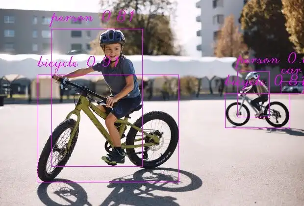
print(results.shape)(45, 6)看起來現(xiàn)在我們有了45個檢測,每個檢測有6個參數(shù)。它們是邊界框的左上角(x1, y1)和右下角(x2, y2)坐標、類別ID和置信度值。在我們繼續(xù)之前,讓我們看一下我運行推理的圖片。

看著這張圖片,人們很容易看出這張圖片中并沒有45個對象。我們的結果矩陣仍然包含這么多檢測的原因是因為多個檢測指向同一個對象。為了解決這個問題,我們可以應用一種眾所周知的技術,稱為非最大抑制(NMS)。NMS充當過濾器,選擇那些可能指向同一對象的最佳檢測。它通過考慮兩個關鍵指標來實現(xiàn)這一點:置信度值(模型對檢測的確定性)和交并比(IOU)。
此外,我們還需要將剩余的檢測結果重新縮放到原始比例。這是因為我們的模型輸出的檢測結果是針對640x640大小的圖像,而不是我們原始圖像的大小。
def NMS(boxes, conf_scores, iou_thresh = 0.55):

    #  boxes [[x1,y1, x2,y2], [x1,y1, x2,y2], ...]

    x1 = boxes[:,0]
    y1 = boxes[:,1]
    x2 = boxes[:,2]
    y2 = boxes[:,3]

    areas = (x2-x1)*(y2-y1)

    order = conf_scores.argsort()

    keep = []
    keep_confidences = []

    while len(order) > 0:
        idx = order[-1]
        A = boxes[idx]
        conf = conf_scores[idx]

        order = order[:-1]

        xx1 = np.take(x1, indices= order)
        yy1 = np.take(y1, indices= order)
        xx2 = np.take(x2, indices= order)
        yy2 = np.take(y2, indices= order)

        keep.append(A)
        keep_confidences.append(conf)

        # iou = inter/union

        xx1 = np.maximum(x1[idx], xx1)
        yy1 = np.maximum(y1[idx], yy1)
        xx2 = np.minimum(x2[idx], xx2)
        yy2 = np.minimum(y2[idx], yy2)

        w = np.maximum(xx2-xx1, 0)
        h = np.maximum(yy2-yy1, 0)

        intersection = w*h

        # union = areaA + other_areas - intesection
        other_areas = np.take(areas, indices= order)
        union = areas[idx] + other_areas - intersection

        iou = intersection/union

        boleans = iou < iou_thresh

        order = order[boleans]

        # order = [2,0,1]  boleans = [True, False, True]
        # order = [2,1]

    return keep, keep_confidences


def rescale_back(results,img_w,img_h):
    cx, cy, w, h, class_id, confidence = results[:,0], results[:,1], results[:,2], results[:,3], results[:,4], results[:,-1]
    cx = cx/640.0 * img_w
    cy = cy/640.0 * img_h
    w = w/640.0 * img_w
    h = h/640.0 * img_h
    x1 = cx - w/2
    y1 = cy - h/2
    x2 = cx + w/2
    y2 = cy + h/2

    boxes = np.column_stack((x1, y1, x2, y2, class_id))
    keep, keep_confidences = NMS(boxes,confidence)
    print(np.array(keep).shape)
    return keep, keep_confidences
其中,`rescaled_results`包含邊界框(x1, y1, x2, y2)和類別ID,而`confidences`存儲相應的置信度分數(shù)。最后,我們準備在圖像上可視化這些結果。
for res, conf in zip(rescaled_results, confidences):

    x1,y1,x2,y2, cls_id = res
    cls_id = int(cls_id)
    x1, y1, x2, y2 = int(x1), int(y1), int(x2), int(y2)
    conf = "{:.2f}".format(conf)
    # draw the bounding boxes
    cv2.rectangle(image,(int(x1),int(y1)),(int(x2),int(y2)),(255,0,255),1)
    cv2.putText(image,classes[cls_id]+' '+conf,(x1,y1-17),
                cv2.FONT_HERSHEY_SCRIPT_COMPLEX,1,(255,0,255),1)