[[190464]]

在梯度下降算法理論篇中，曾經感嘆推導過程如此蒼白，如此期待仿真來給我更加直觀的感覺。當我昨晚Octave仿真后，那種成就感著實難以抑制。分享一下仿真的過程和結果，并且將上篇中未理解透澈的內容補上。

在Gradient Descent Algorithm中，我們利用不斷推導得到兩個對此算法非常重要的公式，一個是J(θ)的求解公式，另一個是θ的求解公式：

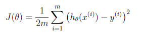
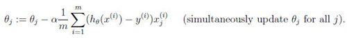
我們在仿真中，直接使用這兩個公式，來繪制J(θ)的分布曲面，以及θ的求解路徑。

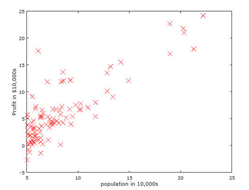
命題為：我們為一家連鎖餐飲企業新店開張的選址進行利潤估算，手中掌握了該連鎖集團所轄店鋪當地人口數據，及利潤金額，需要使用線性回歸算法來建立人口與利潤的關系，進而為新店進行利潤估算，以評估店鋪運營前景。

首先我們將該企業的數據繪制在坐標圖上，如下圖所示，我們需要建立的模型是一條直線，能夠在最佳程度上，擬合population與profit之間的關系。其模型為：

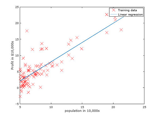
在逼近θ的過程中，我們如下實現梯度下降：進行了1500次的迭代(相當于朝著最佳擬合點行走1500步)，我們在1500步后，得到θ=[-3.630291,1.166362];在3000次迭代后，其值為[-3.878051,1.191253];而如果運行10萬次，其值為[-3.895781，1.193034]。可見，最初的步子走的是非常大的，而后，由于距離最佳擬合點越來越近，梯度越來越小，所以步子也會越來越小。為了節約運算時間，1500步是一個完全夠用的迭代次數。之后，我們繪制出擬合好的曲線，可以看得出，擬合程度還是不錯的。

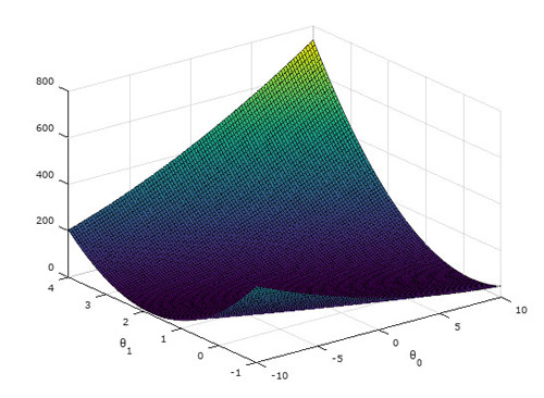
下圖是J(θ)的分布曲面：

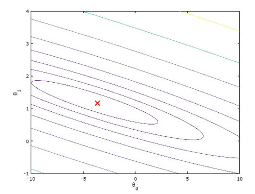
接來下是我們求得的最佳θ值在等高線圖上所在的位置，和上一張圖其實可以重合在一起：

關鍵代碼如下：

1、計算j(theta)

function J = computeCost(X, y, theta) 
%COMPUTECOST Compute cost for linear regression 
%   J = COMPUTECOST(X, y, theta) computes the cost of using theta as the 
%   parameter for linear regression to fit the data points in X and y 
  
% Initialize some useful values 
m = length(y); % number of training examples 
  
% You need to return the following variables correctly 
J = 0; 
  
% ====================== YOUR CODE HERE ====================== 
% Instructions: Compute the cost of a particular choice of theta 
%               You should set J to the cost. 
    h = X*theta; 
    e = h-y; 
    J = e'*e/(2*m) 
% ========================================================================= 
  
end 

2、梯度下降算法：

function [theta, J_history] = gradientDescent(X, y, theta, alpha, num_iters) 
%GRADIENTDESCENT Performs gradient descent to learn theta 
%   theta = GRADIENTDESENT(X, y, theta, alpha, num_iters) updates theta by 
%   taking num_iters gradient steps with learning rate alpha 
  
% Initialize some useful values 
m = length(y); % number of training examples 
J_history = zeros(num_iters, 1); 
  
for iter = 1:num_iters 
  
    % ====================== YOUR CODE HERE ====================== 
    % Instructions: Perform a single gradient step on the parameter vector 
    %               theta. 
    % 
    % Hint: While debugging, it can be useful to print out the values 
    %       of the cost function (computeCost) and gradient here. 
    % 
      
    h=X*theta; 
    e=h-y; 
    theta = theta-alpha*(X'*e)/m; 
  
    % ============================================================ 
  
    % Save the cost J in every iteration    
    J_history(iter) = computeCost(X, y, theta); 
  
end 
  
end