對于深度學習這種端到端模型來說，如何說明和理解其中的訓練過程是大多數研究者關注熱點之一，這個問題對于那種高風險行業顯得尤為重視，比如醫療、軍事等。在深度學習中，這個問題被稱作“黑匣子（Black Box）”。如果不能解釋模型的工作過程，我們怎么能夠就輕易相信模型的輸出結果呢？

以深度學習模型檢測癌癥腫瘤為例，該模型告訴你它能夠檢測出癌癥的準確率高達99%，但它并沒有告訴你它是如何工作并給出判斷結果的。那么該模型是在核磁共振掃描片子中發現了重要線索嗎？或者僅僅是將掃描結果上的污點錯誤地認為是腫瘤呢？模型的輸出結果關系到病人的生死問題及治療方案，醫生是不能承擔起這種錯誤的。

[[224830]]

在本文中，將探討如何可視化卷積神經網絡（CNN），該網絡在計算機視覺中使用最為廣泛。首先了解CNN模型可視化的重要性，其次介紹可視化的幾種方法，同時以一個用例幫助讀者更好地理解模型可視化這一概念。

1.卷積神經網絡模型可視化的重要性

正如上文中介紹的癌癥腫瘤診斷案例所看到的，研究人員需要對所設計模型的工作原理及其功能掌握清楚，這點至關重要。一般而言，一名深度學習研究者應該記住以下幾點：

1. 理解模型是如何工作的

2. 調整模型的參數

3. 找出模型失敗的原因

4. 向消費者/終端用戶或業務主管解釋模型做出的決定

現在讓我們看一個例子，可視化一個神經網絡模型有助于理解其工作原理和提升模型性能。

曾幾何時，美國陸軍希望使用神經網絡自動檢測偽裝的敵方坦克。研究人員使用50張迷彩坦克照片及50張樹林照片來訓練一個神經網絡。使用有監督學習方法來訓練模型，當研究人員訓練好網絡的參數后，網絡模型能夠對訓練集做出正確的判斷——50張迷彩坦克全都輸出“Yes”，50張樹林照片全都輸出“No”。但是這并不能保證模型對于新的樣本也能正確分類。聰明的是，研究人員最初拍攝了200張照片，其中包含了100張迷彩坦克照片、100張樹木照片。從中分別選取50張照片合計100張照片作為訓練集，剩余的100張照片作為測試集。結果發現，模型對測試集也能正確分類。因此，研究人員覺得模型沒有問題了，就將最終成果交付給軍方。原以為軍方會很滿意這份研究成果，結果軍方做出的反饋是他們進行測試后發現效果并不好。

[[224831]]

研究人員感覺此事有點蹊蹺，為什么之前測試時百分百準確，而軍方測試的時候又掉鏈子了呢？最后終于發現，原來是研究者的數據集出現了問題，采集迷彩坦克的時候是陰天，而采集樹林的時候是晴天，神經網絡最終學會的是區分晴天和陰天，而不是區分迷彩坦克和樹林。這真是令人哭笑不得啊，那造成這個問題的主要原因還是沒有弄清楚模型的具體的工作原理及其功能。

2.可視化CNN模型的方法

根據其內部的工作原理，大體上可以將CNN可視化方法分為以下三類：

1.初步方法：一種顯示訓練模型整體結構的簡單方法

2.基于激活的方法：對單個或一組神經元的激活狀態進行破譯以了解其工作過程

3.基于梯度的方法：在訓練過程中操作前向傳播和后向傳播形成的梯度

下面將具體介紹以上三種方法，所舉例子是使用Keras深度學習庫實現，另外本文使用的數據集是由“識別數字”競賽提供。因此，讀者想復現文中案例時，請確保安裝好Kears以及執行了這些步驟。

1初步方法

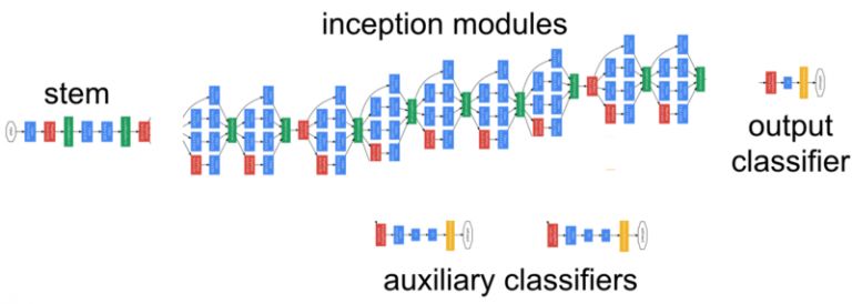
1.1 繪制模型結構圖

研究者能做的最簡單的事情就是繪制出模型結構圖，此外還可以標注神經網絡中每層的形狀及參數。在keras中，可以使用如下命令完成模型結構圖的繪制： 

model.summary()  
_________________________________________________________________  
Layer (type)                 Output Shape              Param #     
=================================================================  
conv2d_1 (Conv2D)            (None, 26, 26, 32)        320        
_________________________________________________________________  
conv2d_2 (Conv2D)            (None, 24, 24, 64)        18496       
_________________________________________________________________ 
max_pooling2d_1 (MaxPooling2 (None, 12, 12, 64)        0     
_________________________________________________________________  
dropout_1 (Dropout)          (None, 12, 12, 64)        0        
_________________________________________________________________  
flatten_1 (Flatten)          (None, 9216)              0        
_________________________________________________________________  
dense_1 (Dense)              (None, 128)               1179776     
_________________________________________________________________  
dropout_2 (Dropout)          (None, 128)               0          
_________________________________________________________________  
preds (Dense)                (None, 10)                1290        
=================================================================  
Total params: 1,199,882  
Trainable params: 1,199,882  
Non-trainable params: 0 

還可以用一個更富有創造力和表現力的方式呈現模型結構框圖，可以使用keras.utils.vis_utils函數完成模型體系結構圖的繪制。

1.2 可視化濾波器

另一種方法是繪制訓練模型的過濾器，這樣就可以了解這些過濾器的表現形式。例如，第一層的第一個過濾器看起來像： 

top_layer = model.layers[0]  
plt.imshow(top_layer.get_weights()[0][:, :, :, 0].squeeze(), cmap='gray') 

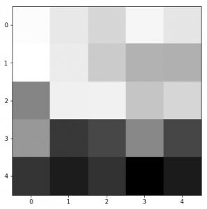
一般來說，神經網絡的底層主要是作為邊緣檢測器，當層數變深時，過濾器能夠捕捉更加抽象的概念，比如人臉等。 

2.激活方法

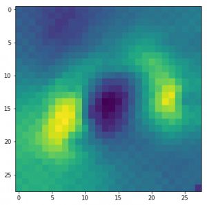
2.1 最大化激活

為了理解神經網絡的工作過程，可以在輸入圖像上應用過濾器，然后繪制其卷積后的輸出，這使得我們能夠理解一個過濾器其特定的激活模式是什么。比如，下圖是一個人臉過濾器，當輸入圖像是人臉圖像時候，它就會被激活。 

from vis.visualization import visualize_activation  
from vis.utils import utils  
from keras import activations  
from matplotlib import pyplot as plt  
%matplotlib inline  
plt.rcParams['figure.figsize'] = (18, 6)  
# Utility to search for layer index by name.  
# Alternatively we can specify this as -1 since it corresponds to the last layer.  
layer_idx = utils.find_layer_idx(model, 'preds')  
# Swap softmax with linear  
model.layers[layer_idx].activation = activations.linear  
model = utils.apply_modifications(model)  
# This is the output node we want to maximize.filter_idx = 0  
img = visualize_activation(model, layer_idx, filter_indices=filter_idx)  
plt.imshow(img[..., 0]) 

同理，可以將這個想法應用于所有的類別，并檢查它們的模式會是什么樣子。 

for output_idx in np.arange(10):  
  # Lets turn off verbose output this time to avoid clutter and just see the output.  
  img = visualize_activation(model, layer_idx, filter_indices=output_idx, input_range=(0., 1.))  
  plt.figure()  
  plt.title('Networks perception of {}'.format(output_idx))  
  plt.imshow(img[..., 0]) 

2.2 圖像遮擋

在圖像分類問題中，可能會遇到目標物體被遮擋，有時候只有物體的一小部分可見的情況。基于圖像遮擋的方法是通過一個灰色正方形系統地輸入圖像的不同部分并監視分類器的輸出。這些例子清楚地表明模型在場景中定位對象時，若對象被遮擋，其分類正確的概率顯著降低。

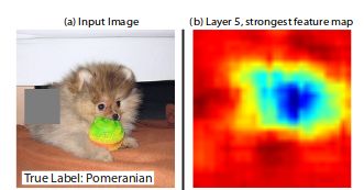
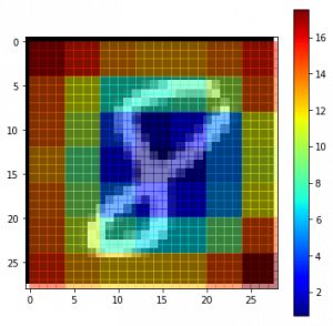
為了理解這一概念，可以從數據集中隨機抽取圖像，并嘗試繪制該圖的熱圖（heatmap）。這使得我們直觀地了解圖像的哪些部分對于該模型而言的重要性，以便對實際類別進行明確的區分。 

def iter_occlusion(image, size=8):  
   # taken from https://www.kaggle.com/blargl/simple-occlusion-and-saliency-maps  
 
  occlusion = np.full((size * 5, size * 5, 1), [0.5], np.float32)  
  occlusion_center = np.full((size, size, 1), [0.5], np.float32)  
  occlusion_padding = size * 2  
 
  # print('padding...')  
  image_padded = np.pad(image, ( \   (occlusion_padding, occlusion_padding), (occlusion_padding, occlusion_padding), (0, 0) \   ), 'constant', constant_values = 0.0)  
 
  for y in range(occlusion_padding, image.shape[0] + occlusion_padding, size):   
      for x in range(occlusion_padding, image.shape[1] + occlusion_padding, size):  
          tmp = image_padded.copy()   
 
          tmp[y - occlusion_padding:y + occlusion_center.shape[0] + occlusion_padding, \  
            x - occlusion_padding:x + occlusion_center.shape[1] + occlusion_padding] \             = occlusion  
 
          tmp[y:y + occlusion_center.shape[0], x:x + occlusion_center.shape[1]] = occlusion_center           yield x - occlusion_padding, y - occlusion_padding, \  
            tmp[occlusion_padding:tmp.shape[0] - occlusion_padding, occlusion_padding:tmp.shape[1] - occlusion_padding]i = 23 # for exampledata = val_x[i]correct_class = np.argmax(val_y[i])  
 
# input tensor for model.predictinp = data.reshape(1, 28, 28, 1)# image data for matplotlib's imshowimg = data.reshape(28, 28)  
# occlusionimg_size = img.shape[0]   
 
occlusion_size = 4print('occluding...')heatmap = np.zeros((img_size, img_size), np.float32)class_pixels = np.zeros((img_size, img_size), np.int16)  
from collections import defaultdict  
counters = defaultdict(int)for n, (x, y, img_float) in enumerate(iter_occlusion(data, size=occlusion_size)):   
   X = img_float.reshape(1, 28, 28, 1)  
   out = model.predict(X)  
   #print('#{}: {} @ {} (correct class: {})'.format(n, np.argmax(out), np.amax(out), out[0][correct_class]))  
   #print('x {} - {} | y {} - {}'.format(x, x + occlusion_size, y, y + occlusion_size))   
   heatmap[y:y + occlusion_size, x:x + occlusion_size] = out[0][correct_class]  
   class_pixels[y:y + occlusion_size, x:x + occlusion_size] = np.argmax(out)  
   counters[np.argmax(out)] += 1 

3. 基于梯度的方法

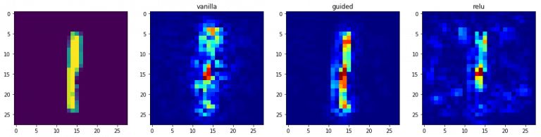
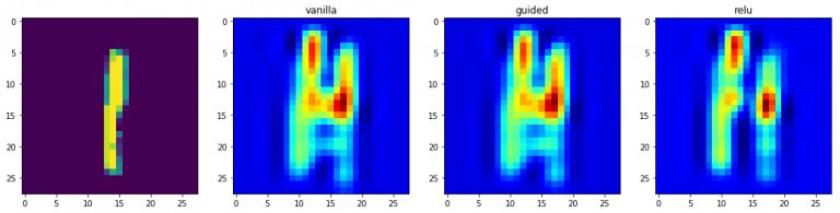
3.1 顯著圖

正如之前的坦克案例中看到的那樣，怎么才能知道模型側重于哪部分的預測呢？為此，可以使用顯著圖解決這個問題。顯著圖首先在這篇文章中被介紹。

使用顯著圖的概念相當直接——計算輸出類別相對于輸入圖像的梯度。這應該告訴我們輸出類別值對于輸入圖像像素中的微小變化是怎樣變化的。梯度中的所有正值告訴我們，像素的一個小變化會增加輸出值。因此，將這些梯度可視化可以提供一些直觀的信息，這種方法突出了對輸出貢獻最大的顯著圖像區域。 

class_idx = 0indices = np.where(val_y[:, class_idx] == 1.)[0]  
# pick some random input from here.idx = indices[0]  
# Lets sanity check the picked image.from matplotlib import pyplot as plt%matplotlib inline  
plt.rcParams['figure.figsize'] = (18, 6)plt.imshow(val_x[idx][..., 0])  
 
from vis.visualization import visualize_saliency  
from vis.utils import utilsfrom keras import activations# Utility to search for layer index by name.  
# Alternatively we can specify this as -1 since it corresponds to the last layer.  
layer_idx = utils.find_layer_idx(model, 'preds')  
# Swap softmax with linearmodel.layers[layer_idx].activation = activations.linear  
model = utils.apply_modifications(model)grads = visualize_saliency(model, layer_idx, filter_indices=class_idx, seed_input=val_x[idx])  
 
# Plot with 'jet' colormap to visualize as a heatmap.plt.imshow(grads, cmap='jet')  
 
# This corresponds to the Dense linear layer.for class_idx in np.arange(10):   
   indices = np.where(val_y[:, class_idx] == 1.)[0]  
   idx = indices[0]  
 
   f, ax = plt.subplots(1, 4)  
   ax[0].imshow(val_x[idx][..., 0])  
 
   for i, modifier in enumerate([None, 'guided', 'relu']):  
       grads = visualize_saliency(model, layer_idx, filter_indices=class_idx,   
       seed_input=val_x[idx], backprop_modifier=modifier)  
       if modifier is None:  
           modifier = 'vanilla'  
       ax[i+1].set_title(modifier)   
       ax[i+1].imshow(grads, cmap='jet') 

3.2 基于梯度的類別激活映射

類別激活映射（CAM）或grad-CAM是另外一種可視化模型的方法，這種方法使用的不是梯度的輸出值，而是使用倒數第二個卷積層的輸出，這樣做是為了利用存儲在倒數第二層的空間信息。 

from vis.visualization import visualize_cam  
# This corresponds to the Dense linear layer.for class_idx in np.arange(10):   
indices = np.where(val_y[:, class_idx] == 1.)[0]  
idx = indices[0]f, ax = plt.subplots(1, 4)  
ax[0].imshow(val_x[idx][..., 0])  
for i, modifier in enumerate([None, 'guided', 'relu']):  
   grads = visualize_cam(model, layer_idx, filter_indices=class_idx,   
   seed_input=val_x[idx], backprop_modifier=modifier)   
   if modifier is None:  
       modifier = 'vanilla'  
   ax[i+1].set_title(modifier)   
   ax[i+1].imshow(grads, cmap='jet') 

總結 

本文簡單說明了CNN模型可視化的重要性，以及介紹了一些可視化CNN網絡模型的方法，希望對讀者有所幫助，使其能夠在后續深度學習應用中構建更好的模型。