三大指標助力K均值與層次聚類數選定及Python示例代碼
在數據分析和機器學習領域,聚類作為一種核心技術,對于從未標記數據中發現模式和洞察力至關重要。聚類的過程是將數據點分組,使得同組內的數據點比不同組的數據點更相似,這在市場細分到社交網絡分析的各種應用中都非常重要。然而,聚類最具挑戰性的方面之一在于確定最佳聚類數,這一決策對分析質量有著重要影響。
雖然大多數數據科學家依賴肘部圖和樹狀圖來確定K均值和層次聚類的最佳聚類數,但還有一組其他的聚類驗證技術可以用來選擇最佳的組數(聚類數)。我們將在sklearn.datasets.load_wine問題上使用K均值和層次聚類來實現一組聚類驗證指標。以下的大多數代碼片段都是可重用的,可以在任何數據集上使用Python實現。
接下來我們主要介紹以下主要指標:
- Gap統計量(Gap Statistics)(!pip install --upgrade gap-stat[rust])
- Calinski-Harabasz指數(Calinski-Harabasz Index )(!pip install yellowbrick)
- Davies Bouldin評分(Davies Bouldin Score )(作為Scikit-Learn的一部分提供)
- 輪廓評分(Silhouette Score )(!pip install yellowbrick)
引入包和加載數據
# Libraries to help with reading and manipulating data
import pandas as pd
import numpy as np
# libaries to help with data visualization
import matplotlib.pyplot as plt
import seaborn as sns
# Removes the limit for the number of displayed columns
pd.set_option("display.max_columns", None)
# Sets the limit for the number of displayed rows
pd.set_option("display.max_rows", 200)
# to scale the data using z-score
from sklearn.preprocessing import StandardScaler
# to compute distances
from scipy.spatial.distance import cdist, pdist
# to perform k-means clustering and compute silhouette scores
from sklearn.cluster import KMeans
from sklearn.metrics import silhouette_score
# to visualize the elbow curve and silhouette scores
from yellowbrick.cluster import KElbowVisualizer, SilhouetteVisualizer
# to perform hierarchical clustering, compute cophenetic correlation, and create dendrograms
from sklearn.cluster import AgglomerativeClustering
from scipy.cluster.hierarchy import dendrogram, linkage, cophenet
sns.set(color_codes=True)


from sklearn.datasets import load_iris, load_wine, load_digits, make_blobs
wine = load_wine()
X_wine = wine.data
X_wine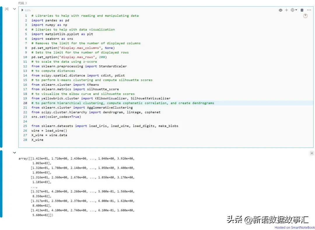
標準化數據:
scaler=StandardScaler()
X_wine_int=X_wine.copy()
X_wine_interim=scaler.fit_transform(X_wine_int)
X_wine_scaled=pd.DataFrame(X_wine_interim)
X_wine_scaled.head(10)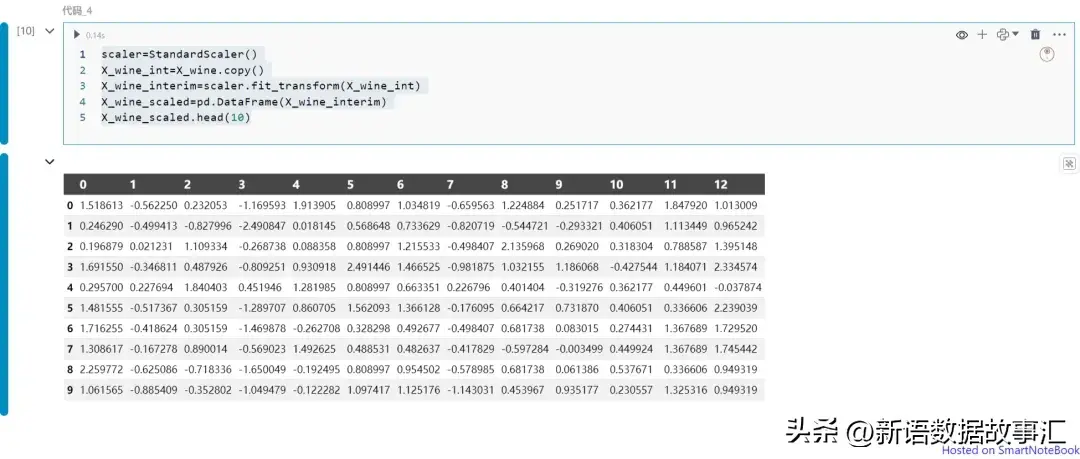
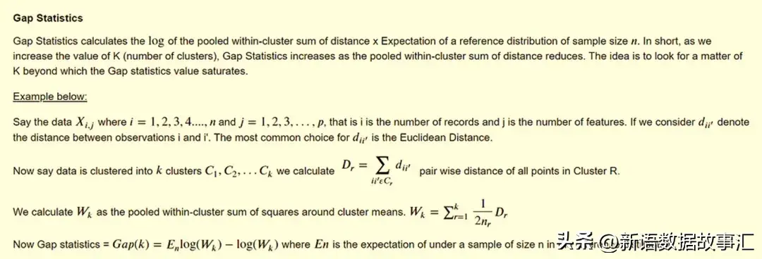
Gap統計量(Gap Statistics)
from gap_statistic import OptimalK
from sklearn.cluster import KMeans
def KMeans_clustering_func(X, k):
    """
    K Means Clustering function, which uses the K Means model from sklearn.
    These user-defined functions *must* take the X (input features) and a k
    when initializing OptimalK
    """

    # Include any clustering Algorithm that can return cluster centers

    m = KMeans(random_state=11, n_clusters=k)
    m.fit(X)
    return m.cluster_centers_, m.predict(X)
#--------------------create a wrapper around OptimalK to extract cluster centers and cluster labels
optimalK = OptimalK(clusterer=KMeans_clustering_func)
#--------------------Run optimal K on the input data (subset_scaled_interim) and number of clusters
n_clusters = optimalK(X_wine_scaled, cluster_array=np.arange(1, 15))
print('Optimal clusters: ', n_clusters)
#--------------------Gap Statistics data frame
optimalK.gap_df[['n_clusters', 'gap_value']]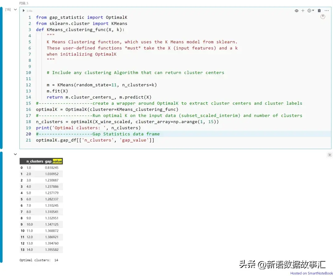
plt.figure(figsize=(10,6))
n_clusters=3
plt.plot(optimalK.gap_df.n_clusters.values, optimalK.gap_df.gap_value.values, linewidth=2)
plt.scatter(optimalK.gap_df[optimalK.gap_df.n_clusters == n_clusters].n_clusters,
            optimalK.gap_df[optimalK.gap_df.n_clusters == n_clusters].gap_value, s=250, c='r')
plt.grid(True)
plt.xlabel('Cluster Count')
plt.ylabel('Gap Value')
plt.title('Gap Values by Cluster Count')
plt.axvline(3, linestyle="--")
plt.show()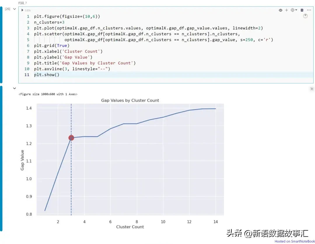
上圖展示不同K值(從K=1到14)下的Gap統計量值。請注意,在本例中我們可以將K=3視為最佳的聚類數。如上所述,可以從圖中獲得Gap統計量的拐點。
Calinski-Harabasz指數(Calinski-Harabasz Inde)
Calinski-Harabasz指數,也稱為方差比準則,是所有組的組間距離與組內距離之和(群內距離)的比值。較高的分數表示更好的聚類緊密度。可以使用Python的YellowBrick庫中的KElbow visualizer來計算。
plt.figure(figsize=(10,6))
model = KMeans(random_state=1)
# k is a range of the number of clusters.
visualizer = KElbowVisualizer(
    model, k=(2, 10), metric="calinski_harabasz", timings=True
)
visualizer.fit(X_wine_scaled)  # Fit the data to the visualizer
visualizer.show()  # Finalize and generate the plot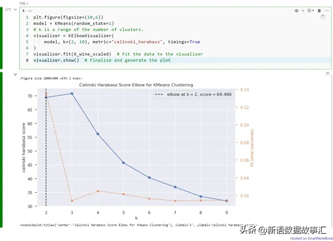
上圖展示不同K值(從K=1到9)下的Calinski Harabasz指數。請注意,在本例中我們可以將K=2視為最佳的聚類數。如上所述,可以從圖中獲得Calinski Harabasz指數的最大值。
使用“metric”超參數選擇用于評估群組的評分指標。默認使用的指標是均方失真,定義為每個點到其最近質心(即聚類中心)的距離平方和。其他一些指標包括:
- distortion:點到其聚類中心的距離平方和的均值
- silhouette:聚類內距離與數據點到其最近聚類中心距離的比率,對所有數據點求平均
- calinski_harabasz:群內到群間離散度的比率
Davies-Bouldin指數(Davies-Bouldin Index)
Davies-Bouldin指數計算為每個聚類(例如Ci)與其最相似聚類(例如Cj)的平均相似度。這個指數表示聚類的平均“相似度”,其中相似度是一種將聚類距離與聚類大小相關聯的度量。具有較低Davies-Bouldin指數的模型在聚類之間有更好的分離效果。對于聚類i到其最近的聚類j的相似度R定義為(Si + Sj) / Dij,其中Si是聚類i中每個點到其質心的平均距離,Dij是聚類i和j質心之間的距離。一旦計算了相似度(例如i = 1, 2, 3, ..., k)到j,我們取R的最大值,然后按聚類數k進行平均。
from sklearn.metrics import davies_bouldin_score
def get_Hmeans_score(  data, distance, link, center):
    """
    returns the  score regarding Davies Bouldin for points to centers
    INPUT:
        data - the dataset you want to fit Agglomerative to
        distance - the distance for AgglomerativeClustering
        link - the linkage method for AgglomerativeClustering
        center - the number of clusters you want (the k value)
    OUTPUT:
        score - the Davies Bouldin score for the Hierarchical model fit to the data
    """
    hmeans = AgglomerativeClustering(n_clusters=center,linkage=link)
    model = hmeans.fit_predict(data)
    score = davies_bouldin_score(data, model)
    return score


centers = list(range(2, 10)) #------Number of Clusters in the data
avg_scores = []
for center in centers:
  avg_scores.append(get_Hmeans_score(X_wine_scaled, "euclidean", "average", center))
plt.figure(figsize=(15,6));

plt.plot(centers, avg_scores, linestyle="-", marker="o", color="b")
plt.xlabel("K")
plt.ylabel("Davies Bouldin score")
plt.title("Davies Bouldin score vs. K")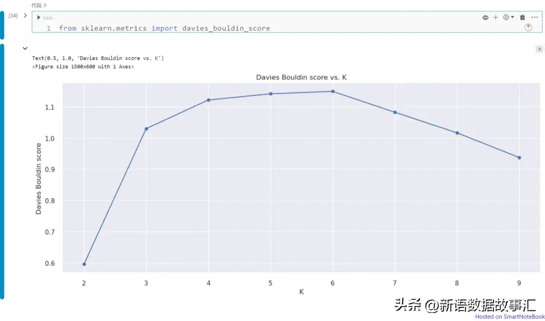
上圖展示不同K值(從K=1到9)下的Davies Bouldin指數。請注意,在本例中我們可以將K=2視為最佳的聚類數。如上所述,可以從圖中獲得Davies Bouldin指數的最小值,該值對應于最優化的聚類數。
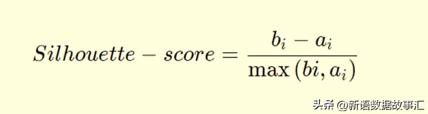
輪廓分數(Silhouette Score)
輪廓分數衡量了考慮到聚類內部(within)和聚類間(between)距離的聚類之間的差異性。在下面的公式中,bi代表了點i到所有不屬于其所在聚類的任何其他聚類中所有點的平均最短距離;ai是所有數據點到其聚類中心的平均距離。如果bi大于ai,則表示該點與其相鄰聚類分離良好,但與其聚類內的所有點更接近。
plt.figure(figsize=(10,6))
model = KMeans(random_state=1)
# k is a range of the number of clusters.
visualizer = KElbowVisualizer(
    model, k=(2, 10), metric="silhouette", timings=True
)
visualizer.fit(X_wine_scaled)  # Fit the data to the visualizer
visualizer.show()  # Finalize and generate the plot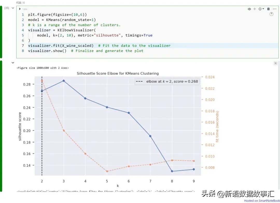
上圖展示不同K值(從K=1到9)下的輪廓分數。請注意,在本例中我們可以將K=2視為最佳的聚類數。如上所述,輪廓分數可以從圖中獲得最大值,該值對應于最優化的聚類數。
在數據分析和機器學習中,聚類是一項關鍵技術,幫助我們從未標記的數據中發現模式和洞察。確定最佳聚類數是聚類過程中的重要挑戰,影響分析質量。本文介紹了多種聚類驗證技術如Gap統計量、Calinski-Harabasz指數、Davies Bouldin指數和輪廓分數,這些指標可以幫助我們選擇最優化的聚類數,提升聚類結果的有效性和可靠性。