在 CIFAR10 數據集上訓練 Vision Transformer (ViT)

在這篇簡短的文章中,我將構建一個簡單的 ViT 并將其訓練在 CIFAR 數據集上。
訓練循環
我們從訓練 CIFAR 數據集上的模型的樣板代碼開始。我們選擇批量大小為64,以在性能和 GPU 資源之間取得平衡。我們將使用 Adam 優化器,并將學習率設置為0.001。與 CNN 相比,ViT 收斂得更慢,所以我們可能需要更多的訓練周期。此外,根據我的經驗,ViT 對超參數很敏感。一些超參數會使模型崩潰并迅速達到零梯度,模型的參數將不再更新。因此,您必須測試與模型大小和形狀本身以及訓練超參數相關的不同超參數。
transform_train = transforms.Compose([
    transforms.Resize(32),
    transforms.ToTensor(),
    transforms.Normalize((0.4914, 0.4822, 0.4465), (0.2023, 0.1994, 0.2010)),
])

transform_test = transforms.Compose([
    transforms.Resize(32),
    transforms.ToTensor(),
    transforms.Normalize((0.4914, 0.4822, 0.4465), (0.2023, 0.1994, 0.2010)),
])

train_set = CIFAR10(root='./datasets', train=True, download=True, transform=transform_train)
test_set = CIFAR10(root='./datasets', train=False, download=True, transform=transform_test)

train_loader = DataLoader(train_set, shuffle=True, batch_size=64)
test_loader = DataLoader(test_set, shuffle=False, batch_size=64)
n_epochs = 100
lr = 0.0001
optimizer = Adam(model.parameters(), lr=lr)
criterion = CrossEntropyLoss()
for epoch in range(n_epochs):
train_loss = 0.0
for i,batch in enumerate(train_loader):
x, y = batch
x, y = x.to(device), y.to(device)
y_hat, _ = model(x)
loss = criterion(y_hat, y)
batch_loss = loss.detach().cpu().item()
train_loss += batch_loss / len(train_loader)
optimizer.zero_grad()
loss.backward()
optimizer.step()
if i%100==0:
print(f"Batch {i}/{len(train_loader)} loss: {batch_loss:.03f}")
print(f"Epoch {epoch + 1}/{n_epochs} loss: {train_loss:.03f}")構建 ViT
如果您熟悉注意力和transforms塊,ViT 架構就很容易理解。簡而言之,我們將使用 Pytorch 提供的多頭注意力,視覺transforms的第一部分是將圖像分割成相同大小的塊。如您所知,transforms作用于標記,而不是像在 CNN 中那樣卷積特征。在我們的例子中,圖像塊充當標記。
有很多方法可以對圖像進行分塊。有些人手動進行,這不符合 Python 的風格。其他人使用卷積。還有些人使用 Pytorch 提供的張量操作工具。我們將使用 Pytorch nn 模塊提供的 unfold 層作為我們 Patcher 模塊的核心。
該模塊作用于形狀為 (N, 3, 32, 32) 的張量。其中 N 是每批圖像的數量。3 是通道數,因為我們處理的是 RGB 圖像。32 是圖像的大小,因為我們處理的是 CIFAR10 數據集。我們可以測試我們的模塊,以確保它將上述形狀轉換為分塊張量。新張量的形狀取決于補丁大小。如果我們選擇補丁大小為4,輸出形狀將是 (N, 64, 3, 4, 4),其中 64 是每張圖像的補丁數量。
class Patcher(nn.Module):
  def __init__(self, patch_size):
    super(Patcher, self).__init__()

    self.patch_size=patch_size

    self.unfold = torch.nn.Unfold(kernel_size=patch_size, stride=patch_size)

  def forward(self, images):
    batch_size, channels, height, width = images.shape

    patch_height, patch_width = [self.patch_size, self.patch_size]
    assert height % patch_height == 0 and width % patch_width == 0, "Height and width must be divisible by the patch size."

    patches = self.unfold(images) #bs (cxpxp) N
    patches = patches.view(batch_size, channels, patch_height, patch_width, -1).permute(0, 4, 1, 2, 3) # bs N C P P

    return patches
x = torch.rand((10, 3, 32, 32))
x = Patcher(patch_size=4)(x)
x.shape
# torch.Size([10, 64, 3, 4, 4])在語言處理中,標記通過詞嵌入投影到 d 維向量中。這個超參數 d 是transforms模型的特征,選擇合適的維度大小對于模型的轉換很重要。太大,模型會崩潰。太小,模型將無法很好地訓練。因此,到目前為止,我們的 ViT 模塊形狀將如下所示:
class ViT_RGB(nn.Module):
  def __init__(self, img_size, patch_size, model_dim= 100):
    super().__init__()

    self.img_size = img_size
    self.patch_size = patch_size
    self.n_patches = (self.img_size // self.patch_size) ** 2
    self.model_dim = model_dim

    # 1) Patching
    self.patcher = Patcher(patch_size=self.patch_size)

    # 2) Linear Prjection
    self.linear_projector = nn.Linear( 3 * self.patch_size ** 2, self.model_dim)

  def forward(self, x):

    x = self.patcher(x)

    x = x.flatten(start_dim=2)

    x = self.linear_projector(x)

    return x
我們將圖像 (N, 3, 32, 32) 分割成大小為4的補丁 (N, 64, 3, 4, 4),然后我們將它們展平為 (N, 64, 344=48)。之后,我們使用 Pytorch 的 Linear 模塊將它們投影到大小為 (N, 64, 100)。
即使在將輸入喂入transforms塊之后,整個模塊的輸出大小也將是 (N, n_patches, model_dim)。現在我們有很多投影和關注的補丁,應該使用哪個補丁進行預測?一種常見的方法是計算所有補丁的平均值,然后使用平均向量進行預測。然而,對于transforms,現在正在廣泛使用另一種技巧。那就是添加一個 [cls] 一個新的標記到輸入中。輔助標記最終將用于預測。它將作用于模型對整個圖像的理解。該標記只是一個大小為 (1, model_dim) 的參數向量。現在,整個模塊的輸出將是 (N, n_patches+1, model_dim)。
class ViT_RGB(nn.Module):
  def __init__(self, img_size, patch_size, model_dim= 100):
    super().__init__()
    self.img_size = img_size
    self.patch_size = patch_size
    self.n_patches = (self.img_size // self.patch_size) ** 2
    self.model_dim = model_dim

    # 1) Patching
    self.patcher = Patcher(patch_size=self.patch_size)

    # 2) Linear Prjection
    self.linear_projector = nn.Linear( 3 * self.patch_size ** 2, self.model_dim)

    # 3) Class Token
    self.class_token = nn.Parameter(torch.rand(1, self.model_dim))


  def forward(self, x):

    x = self.patcher(x)

    x = x.flatten(start_dim=2)

    x = self.linear_projector(x)

    batch_size = x.shape[0]
    class_token = self.class_token.expand(batch_size, -1, -1)
    x = torch.cat((class_token, x), dim=1)

    return x
在添加了類標記之后,我們仍然需要添加位置編碼部分。transforms操作在一系列標記上,它們對序列順序視而不見。為了確保在訓練中加入順序,我們手動添加位置編碼。因為我們處理的是大小為 model_dim 的向量,我們不能簡單地添加順序 [0, 1, 2, …],位置應該是模型固有的,這就是為什么我們使用所謂的位置編碼。這個向量可以手動設置或訓練。在我們的例子中,我們將簡單地訓練一個位置嵌入,它只是一個大小為 (1, n_patches+1, model_dim) 的向量。我們將這個向量添加到完整的補丁序列中,以及類標記。如前所述,為了計算模型的輸出,我們簡單地對嵌入的第一個標記(類標記)應用一個帶有 SoftMax 層的 MLP,以獲得類別的對數幾率。
class ViT_RGB(nn.Module):
  def __init__(self, img_size, patch_size, model_dim= 100,n_classes=10):
    super().__init__()
    self.img_size = img_size
    self.patch_size = patch_size
    self.n_patches = (self.img_size // self.patch_size) ** 2
    self.model_dim = model_dim

    # 1) Patching
    self.patcher = Patcher(patch_size=self.patch_size)

    # 2) Linear Prjection
    self.linear_projector = nn.Linear( 3 * self.patch_size ** 2, self.model_dim)

    # 3) Class Token
    self.class_token = nn.Parameter(torch.rand(1, 1, self.model_dim))

    # 4) Positional Embedding
    self.positional_embedding = nn.Parameter(torch.rand(1,(img_size // patch_size) ** 2 + 1, model_dim))

    # 6) Classification MLP
    self.mlp = nn.Sequential(
            nn.Linear(self.model_dim, self.n_classes),
            nn.Softmax(dim=-1)
      )

  def forward(self, x):

    x = self.patcher(x)

    x = x.flatten(start_dim=2)
    x = self.linear_projector(x)

    batch_size = x.shape[0]
    class_token = self.class_token.expand(batch_size, -1, -1)
    x = torch.cat((class_token, x), dim=1)

    x = x + self.positional_embedding

    latent = x[:, 0]
    logits = self.mlp(latent)

    return logits
transforms塊
之前的代碼沒有包括非常重要的transforms塊。transforms塊是大小保持塊,它們通過交叉組成序列的標記本身來豐富信息序列。transforms塊的核心模塊是注意力模塊(同樣,您可以查看我關于注意力的帖子)。為了使模型更豐富地處理信息,我們通常使用多頭注意力。為了使模型吸收越來越抽象的信息,我們應用了幾個transforms塊。使用的頭數和transforms塊的數量是transforms模型的特征。我們稱使用的transforms塊數量為模型的 depth。
class TransformerBlock(nn.Module):
    def __init__(self, model_dim, num_heads, mlp_ratio=4.0, dropout=0.1):
        super(TransformerBlock, self).__init__()
        self.norm1 = nn.LayerNorm(model_dim)
        self.attn = nn.MultiheadAttention(model_dim, num_heads, dropout=dropout)
        self.norm2 = nn.LayerNorm(model_dim)

        # Feedforward network
        self.mlp = nn.Sequential(
            nn.Linear(model_dim, int(model_dim * mlp_ratio)),
            nn.GELU(),
            nn.Linear(int(model_dim * mlp_ratio), model_dim),
            nn.Dropout(dropout),
        )

    def forward(self, x):
        # Self-attention
        x = self.norm1(x)
        attn_out, _ = self.attn(x, x, x)
        x = x + attn_out

        # Feedforward network
        x = self.norm2(x)
        mlp_out = self.mlp(x)
        x = x + mlp_out

        return x
class ViT_RGB(nn.Module):
def __init__(self, img_size, patch_size, model_dim= 100, num_heads=3, num_layers=2, n_classes=10):
super().__init__()
self.img_size = img_size
self.patch_size = patch_size
self.n_patches = (self.img_size // self.patch_size) ** 2
self.model_dim = model_dim
self.num_layers = num_layers
self.num_heads= num_heads
self.n_classes = n_classes
# 1) Patching
self.patcher = Patcher(patch_size=self.patch_size)
# 2) Linear Prjection
self.linear_projector = nn.Linear( 3 * self.patch_size ** 2, self.model_dim)
# 3) Class Token
self.class_token = nn.Parameter(torch.rand(1, 1, self.model_dim))
# 4) Positional Embedding
self.positional_embedding = nn.Parameter(torch.rand(1,(img_size // patch_size) ** 2 + 1, model_dim))
# 5) Transformer blocks
self.blocks = nn.ModuleList([
TransformerBlock( self.model_dim, self.num_heads) for _ in range(num_layers)
])
# 6) Classification MLPk
self.mlp = nn.Sequential(
nn.Linear(self.model_dim, self.n_classes),
nn.Softmax(dim=-1)
)
def forward(self, x):
x = self.patcher(x)
x = x.flatten(start_dim=2)
x = self.linear_projector(x)
batch_size = x.shape[0]
class_token = self.class_token.expand(batch_size, -1, -1)
x = torch.cat((class_token, x), dim=1)
x = x + self.positional_embedding
for block in self.blocks:
x = block(x)
latent = x[:, 0]
logits = self.mlp(latent)
return logits最后,我們為訓練和測試準備好了模型,并放置了所有必要的組件。然而,在實踐中,我無法通過在類標記上應用 MLP 層使模型收斂。我不確定為什么——如果你知道,請告訴我。相反,我在整個圖像補丁的平均向量上應用了 MLP。